101 Excel 2013 Tips, Tricks and Timesavers (39 page)
Read 101 Excel 2013 Tips, Tricks and Timesavers Online
Authors: John Walkenbach

Figure 97-2:
Grouped charts, after resizing the group.
Even though charts are grouped, you can still work with a particular chart in a group — and charts that are in a group can still be moved and resized individually. To work with a single chart in a group, click anywhere in the group to select the group; then click the chart you want to work on.
To ungroup the objects in the group, right-click anywhere in the group and choose Group
➜
Ungroup.
Grouping other objects
You can combine various types of objects into a group. Figure 97-3 shows a group that consists of a shape (which serves as the background), a text box, and a chart. Figure 97-4 shows the group after I resized it to change the proportions. Resizing a group is much easier than resizing three separate objects.
 When combining objects that overlap, you’ll often need to adjust the stack order. Right-click an object and use the Bring to Front or Send to Back commands.
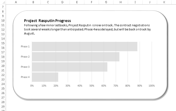
Figure 97-3:
Three objects in a group.
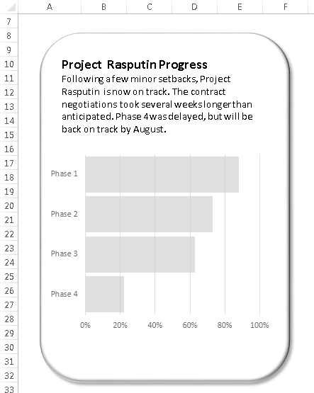
Figure 97-4:
The object group, after resizing.
Tip 98: Taking Pictures of Ranges
Excel makes it easy to convert a range of cells into a picture. The picture can either be a
static
image (it doesn’t change if the original range changes) or a
live
picture (which reflects changes in the original range). The range can even contain objects, such as charts or shapes.
Creating a static image of a range
To create a snapshot of a range, start by selecting a range of cells and then press Ctrl+C to copy the range to the Clipboard. Then choose Home⇒Clipboard⇒Paste⇒Other Paste Options⇒Picture (U). The result is a graphic image of the original range, pasted on top of the original range. Just click and drag to move the picture to another location. When you select this image, Excel displays its Picture Tools context menu — which means that you can apply some additional formatting to the picture.
Figure 98-1 shows a range of cells (B2:E9), along with a picture of the range after I applied one of the built-in styles from the Picture Tools⇒Format⇒Picture Styles gallery. It’s a static picture, so changes made within the range B2:E9 aren’t shown in the picture.
If you want to include a graphic that shows information from another (non-Excel) window, choose Insert⇒Illustrations⇒Screenshot. You can capture an entire window or just a portion of a window (by choosing Screen Clipping). The copied information is pasted as a picture in the active worksheet.
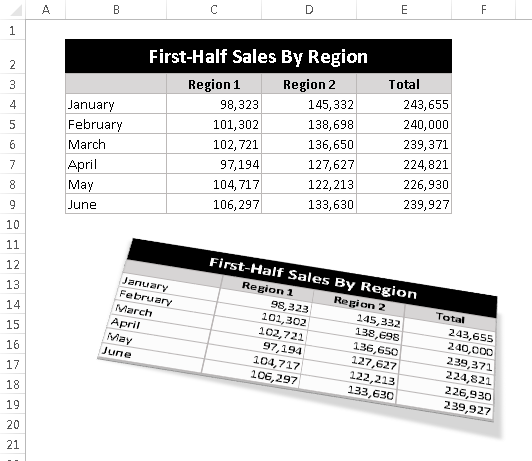
Figure 98-1:
A picture of a range, after applying some picture formatting.
Creating a live image of a range
To create an image that’s linked to the original range of cells, select the cells and press Ctrl+C to copy the range to the Clipboard. Then choose Home⇒Clipboard⇒Paste⇒Other Paste Options⇒Linked Picture (I). Excel pastes a picture of the original range, and the picture is linked — if you make changes to the original, those changes are shown in the linked picture.
Notice that when you select the linked picture, the Formula bar displays the address of the original range. You can edit this range reference to change the cells that are displayed in the picture. To unlink the picture, just delete the formula on the Formula bar.
As with an unlinked picture, you can use Excel’s Picture Tools context menu to modify the appearance of the linked picture.
You can also cut and paste this picture to a different worksheet, if you like. Doing so makes it easy to refer to information on a different sheet.
Figure 98-2 shows a linked picture of a range placed on top of a shape, which has lots of interesting formatting capabilities. Placing a linked picture on top of a shape is a good way to make a particular range stand out.
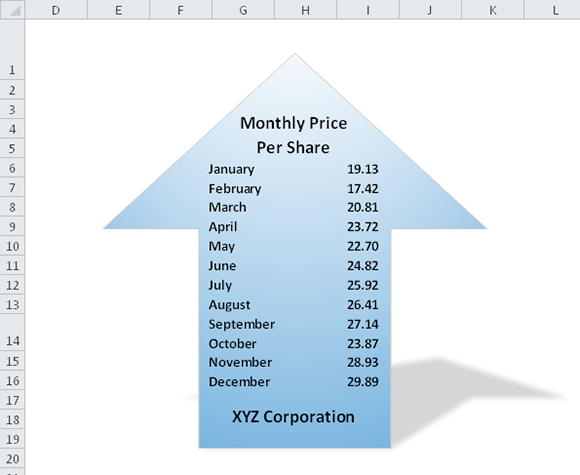
Figure 98-2:
A linked picture of a range, placed on top of a shape.
Saving a range as a graphic image
If you need to save a range as a graphic image, the best approach is to use one of several screen capture programs that are available. This type of software makes it easy to capture complete windows or just a portion of a window. After you capture the screen, click a button to save it as a graphics image in the format you choose (GIF, PNT, TIF, and so on).
If you don’t have a screen capture program, you probably have some other type of graphics software. When you copy a range of cells, that range is stored on the Windows Clipboard in several different formats. One of those formats is a graphic image. Therefore, you can copy a range, activate your graphics software, and press Ctrl+V to paste the range as a graphic. Then save the graphics file in your desired format.
Figure 98-3 shows a range after it was copied and pasted into a freeware program named IrfanView.
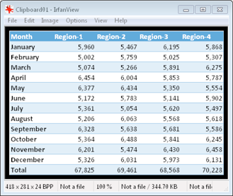
Figure 98-3:
A range of data, ready to be saved as a graphic image.
Copying a range is a what-you-see-is-what-you-get thing. For example, if the selected range contains a chart, the chart will also appear in the image.
 For another method to save a range as a graphic image, see Tip 101.
Tip 99: Changing the Look of Cell Comments
Cell comments are useful for a variety of purposes. But sometimes you just get tired of looking at the same old yellow rectangle. This tip describes three tricks that you can use to make your comments stand out:
→ Format a comment.
→ Change the shape of a comment.
→ Add an image to a comment.
All of these changes require that the cell comment is visible. If the comment isn’t visible, right-click the cell and choose Show/Hide Comments from the shortcut menu.