101 Excel 2013 Tips, Tricks and Timesavers (31 page)
Read 101 Excel 2013 Tips, Tricks and Timesavers Online
Authors: John Walkenbach

Figure 77-2:
A pivot table created from the data.
Figure 77-3 shows an example of an Excel range that is
not
appropriate for a pivot table. Although the range contains descriptive information about each value, it does
not
consist of normalized data, and you cannot create a useful pivot table from it. In fact, this range actually resembles a pivot table summary, but it’s much less flexible.
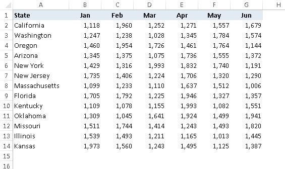
Figure 77-3:
This range is not appropriate for a pivot table.
Figure 77-4 shows the same data, but normalized. This range contains 78 rows of data — one for each of the six monthly sales values for the 13 states. Notice that each row contains category information for the sales value. This table is an ideal candidate for a pivot table and contains all information necessary to summarize the information by region or quarter.
Figure 77-5 shows a pivot table created from the normalized data. As you can see, it’s virtually identical to the non-normalized data shown in Figure 77-3. Working with normalized data provides ultimate flexibility in designing reports.
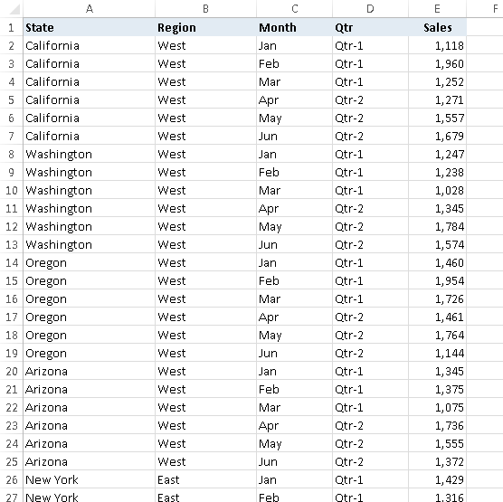
Figure 77-4:
This range contains normalized data and is appropriate for a pivot table.
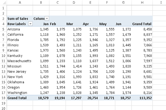
Figure 77-5:
A pivot table created from normalized data.
Tip 78: Using a Pivot Table Instead of Formulas
The Excel PivotTable feature is incredibly powerful, and you can often create pivot tables in lieu of creating formulas. This tip describes a specific problem and provides three different solutions.
Figure 78-1 shows a range of data that contains student test scores. The goal is to calculate the average score for all students plus the average score for each gender.
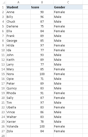
Figure 78-1:
What’s the best way to calculate the average test score for males versus females?
Inserting subtotals
The first solution involves automatically inserting subtotals. To use this method, the data must be sorted by the column that will trigger the subtotaling. In this case, you need to sort by the Gender column. Follow these steps:
1.
Select any cell in column C.
2.
Right-click and choose Sort⇒Sort A to Z from the shortcut menu.
3.
Choose Data⇒Outline⇒Subtotal.
The Subtotal dialog box appears.
4.
Specify At Each Change in Gender, Use Function Average, and Add Subtotal to Score.
The result of adding subtotals is shown in Figure 78-2. Notice that Excel also creates an outline, so you can hide the details and view just the summary.
The formulas inserted by Excel use the SUBTOTAL function, with 1 as the first argument (1 represents average). Here are the formulas:
=SUBTOTAL(1,B2:B13)
=SUBTOTAL(1,B15:B28)
=SUBTOTAL(1,B2:B28)
The formula in cell B30 calculates the Grand Average and uses a range that includes the other two SUBTOTAL formulas in cells B14 and B29. The SUBTOTAL function ignores cells that contain other SUBTOTAL formulas.
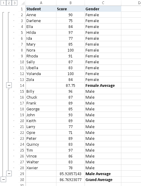
Figure 78-2:
Excel adds subtotals automatically.
Using formulas
Another method of creating averages is to use formulas. The formula to calculate the average of all students is simple:
=AVERAGE(B2:B27)
To calculate the average of the genders, you can use the AVERAGEIF function and create these formulas:
=AVERAGEIF(C2:C27,”Female”,B2:B27)
=AVERAGEIF(C2:C27,”Male”,B2:B27)
Using Excel’s PivotTable feature
A third method of averaging the scores is to create a pivot table. Many users avoid creating pivot tables because they consider this feature too complicated. As you can see, it’s simple to use:
1.
Select any cell in the data range and choose Insert⇒Tables⇒PivotTable.
The Create PivotTable dialog box appears.
2.
Verify that Excel selected the correct data range and specify a cell on the existing worksheet as the location.
Cell E1 is a good choice.
3.
Click OK.
Excel displays the PivotTable Fields task pane.
4.
Drag the Gender item to the Rows section, at the bottom.
5.
Drag the Score item to the Values section.
Excel creates the pivot table but calculates the sum of the scores rather than the average.
6.
To change the summary function that’s used, right-click any of the values in the pivot table and choose Summarize Data By⇒Average from the shortcut menu.
Figure 78-3 shows the pivot table and the PivotTable Fields task pane.
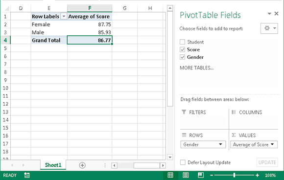
Figure 78-3:
This pivot table calculates the averages without using formulas.
 Unlike a formula-based solution, a pivot table doesn’t update itself automatically if the data changes. If the data changes, you must refresh the pivot table. Just right-click any cell in the pivot table and choose Refresh from the shortcut menu.
The pivot table in this example is extremely simple, but it’s also very easy to create. Pivot tables can be much more complex, and they can summarize massive amounts of data in just about any way you can think of — without using any formulas.
Tip 79: Controlling References to Cells Within a Pivot Table
In some cases, you may want to create a formula that references one or more cells within a pivot table. Figure 79–1 shows a simple pivot table that displays income and expense information for three years. In this pivot table, the Month field is hidden, so the pivot table shows the year totals.
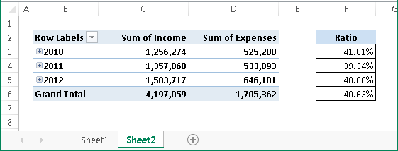
Figure 79-1:
The formulas in column F reference cells in the pivot table.
Column F contains formulas, and this column is not part of the pivot table. These formulas calculate the expense-to-income ratio for each year. I created these formulas by pointing to the cells. You may expect to see this formula in cell F3:
=D3/C3
In fact, the formula in cell F3 is
=GETPIVOTDATA(“Sum of Expenses”,$B$2,”Year”,2010)
/GETPIVOTDATA(“Sum of Income”,$B$2,”Year”,2010)