101 Excel 2013 Tips, Tricks and Timesavers (28 page)
Read 101 Excel 2013 Tips, Tricks and Timesavers Online
Authors: John Walkenbach

Figure 69-3:
A preview of Quick Analysis Sparklines.
 The Quick Analysis options don’t enable you to do anything that you can’t do using Excel’s normal commands. But sometimes it can you save a bit of time. If you find the Quick Analysis button annoying, turn if off in the General tab of the Excel Options dialog box. Deselect the check box labeled Show Quick Analysis Options on Selection.
Tip 70: Filling the Gaps in a Report
When you import data, you can sometimes end up with a worksheet that looks something like the one shown in Figure 70-1. This type of report formatting is common. As you can see, an entry in column A applies to several rows of data. If you sort this type of list, the missing data messes things up, and you can no longer tell who sold what when.
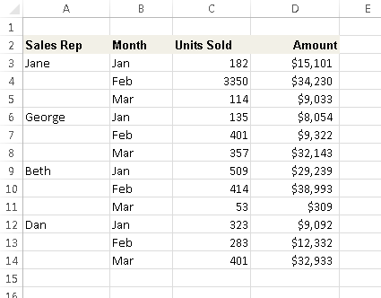
Figure 70-1:
This report contains gaps in the Sales Rep column.
If your list is small, you can enter the missing cell values manually or by using a series of Home
➜
Editing⇒Fill⇒Down commands (or its Ctrl+D shortcut). But if you have a large list that’s in this format, you need a better way of filling in those cell values. Here’s how:
1.
Select the range that has the gaps (A3:A14, in this example).
2.
Choose Home⇒Editing⇒Find & Select⇒Go To Special.
The Go To Special dialog box appears.
3.
Select the Blanks option and click OK.
This action selects the blank cells in the original selection.
4.
On the Formula bar, type an equal sign (
=
) followed by the address of the first cell with an entry in the column (
=A3,
in this example) and press Ctrl+Enter.
5.
Reselect the original range and press Ctrl+C to copy the selection.
6.
Choose Home⇒Clipboard⇒Paste⇒Paste Values to convert the formulas to values.
After you complete these steps, the gaps are filled in with the correct information, and your worksheet looks similar to the one shown in Figure 70-2. Now it’s a normal list, and you can do whatever you like with it — including sorting.

Figure 70-2:
The gaps are gone, and this list can now be sorted.
Tip 71: Performing Inexact Searches
If you have a large worksheet with lots of data, locating what you’re looking for can be difficult. The Excel Find and Replace dialog box is a useful tool for locating information, and it has a few features that many users overlook.
Access the Find and Replace dialog box by choosing Home⇒Editing⇒Find & Select⇒Find (or by pressing Ctrl+F). If you’re replacing information, you can use Home⇒Editing⇒Find & Select⇒Replace (or Ctrl+H). The only difference is which of the two tabs is displayed in the dialog box. Figure 71-1 shows the Find and Replace dialog box after clicking the Options button, which expands the dialog box to show additional options.

Figure 71-1:
The Find and Replace dialog box with the Find tab selected.
In many cases, you want to locate “approximate” text. For example, you may be trying to find data for a customer named Stephen R. Rosencrantz. You can, of course, search for the exact text:
Stephen R. Rosencrantz.
However, there’s a reasonably good chance that the search will fail. The name may have been entered differently, as Steve Rosencrantz or S.R. Rosencrantz, for example. It may have even been misspelled as Rosentcrantz.
The most efficient search for this name is to use a wildcard character and search for st*rosen* and then click the Find All button. In addition to reducing the amount of text that you enter, this search is practically guaranteed to locate the customer, if the record is in your worksheet. The search may also find some records that you aren’t looking for, but that’s better than not finding anything.
The Find and Replace dialog box supports two wildcard characters:
→ ? matches any single character.
→ * matches any number of characters.
Wildcard characters also work with values. For example, searching for 3* locates all cells that contain an entry that begins with 3. Searching for 1?9 locates all three-digit entries that begin with 1 and end with 9.
To search for a question mark or an asterisk, precede the character with a tilde character (~). For example, the following search string finds the text *NONE*:
~*NONE~*
If you need to search for the tilde character, use two tildes.
If your searches don’t seem to be working correctly, double-check these three options (which sometimes have a way of changing on their own):
→
Match Case:
If this check box is selected, the case of the text must match exactly. For example, searching for smith does not locate Smith.
→
Match Entire Cell Contents:
If this check box is selected, a match occurs if the cell contains only the search string (and nothing else). For example, searching for Excel doesn’t locate a cell that contains Microsoft Excel.
→
Look In:
This drop-down list has three options: Values, Formulas, and Comments. If, for example, Values is selected, searching for 900 doesn’t find a cell that contains 900 if that value is generated by a formula.
Remember that searching operates on the selected range of cells. If you want to search the entire worksheet, select only one cell before you begin your search.
Also, remember that searches do not include numeric formatting. For example, if you have a value that uses currency formatting so that it appears as $54.00, searching for $5* doesn’t locate that value.
Working with dates can be a bit tricky because Excel offers many ways to format dates. If you search for a date by using the default date format, Excel locates the dates even if they’re formatted differently. For example, if your system uses the m/d/y date format, the search string 10/*/2013 finds all dates in October 2013, regardless of how the dates are formatted.
You can also use an empty Replace With field. For example, to quickly delete all asterisks from your worksheet, enter
~*
in the Find What field and leave the Replace With field blank. When you click the Replace All button, Excel finds all the asterisks and replaces them with nothing.
Tip 72: Proofing Your Data with Audio
Excel 2002 introduced a handy feature: text-to-speech. In other words, Excel is capable of speaking to you. You can have this feature read back a specific range of cells, or you can set it up so that it reads the data as you enter it.
For some reason, this feature appears to be missing in action, beginning with Excel 2007. You can search the Ribbon all day and not find a trace of the text-to-speech feature. But the feature is still available — you just need to spend a few minutes to make it accessible.
Adding speech commands to the Ribbon
Following are instructions to add these commands to a new group in the Review tab of the Ribbon:
1.
Right-click the Ribbon and then choose Customize the Ribbon from the shortcut menu.
The Customize Ribbon tab of the Excel Options dialog box appears.
2.
In the list box on the right, select Review and click New Group.
3.
Click Rename and overwrite the default name with a more descriptive name, such as Text To Speech.
4.
Click the drop-down list on the left and choose Commands Not in the Ribbon.
5.
Scroll down the list, and you find five items that begin with the word
Speak;
select each one and then click Add.
They’re added to the newly created group (see Figure 72-1).
6.
Click OK to close the Excel Options dialog box.
After you perform these steps, the Review tab displays a new group with five new icons (see Figure 72-2).
Using the speech commands
To read a range of cells, select the range first and then click the Speak Cells button. You can also specify the orientation (By Rows or By Columns). To read the data as it’s entered, click the Speak On Enter button.
Some people (myself included) find the voice in this “love it or hate it” feature much too annoying to use for any extended period. And, if you enter the data at a relatively rapid clip, the voice simply cannot keep up with you.
You have a small bit of control over the voice used in the Excel Text To Speech feature. To adjust the voice, open the Windows Control Panel and display the Text to Speech tab of the Speech Properties dialog box. You can adjust the speed and select a different voice (if other voices are installed). Click the Preview Voice button to help make your choices.
