101 Excel 2013 Tips, Tricks and Timesavers (25 page)
Read 101 Excel 2013 Tips, Tricks and Timesavers Online
Authors: John Walkenbach

=IF(NOT(ISNONTEXT(A1)),A1<>TRIM(A1))
Tip 63: Transposing a Range
You may have a range of data that should be transposed. Transposing a range is essentially making the rows columns, and the columns rows. Figure 63-1 shows an example. The original data is in A1:H9, and the transposed data is in A12:I19.
This tip describes two methods to transpose a range of data.
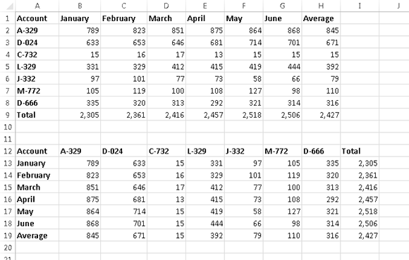
Figure 63-1:
Data before and after being transposed.
Using Paste Special
To transpose a range of data by copying and pasting, follow these steps:
1.
Select the range to be transposed.
2.
Press Ctrl+C to copy the range.
3.
Select the cell that will be the upper-left cell for the transposed range.
4.
Choose Home⇒Clipboard⇒Paste⇒Paste Special to display the Paste Special dialog box.
5.
Choose the Transpose option.
6.
Click OK.
Excel pastes the copied data, but reoriented.
If the original range contains formulas, the formulas will be adjusted so they continue to refer to the correct cells.
 If the original range is in a table (created with Insert⇒Tables⇒Table), this technique has a few caveats. The original selection cannot include the Total Row or columns that contain a formula. You can still paste the transposed data, but you must choose the Values option in the Paste Special dialog box. The transposed range will include the values (but not the formulas).
Using the TRANSPOSE function
In some cases, you may want the transposed range to be linked to the original range. In such a situation, changes made to the original range also appear in the transposed range. Here’s how to set up a transposed range that’s linked to the original source. Refer to Figure 63-2.
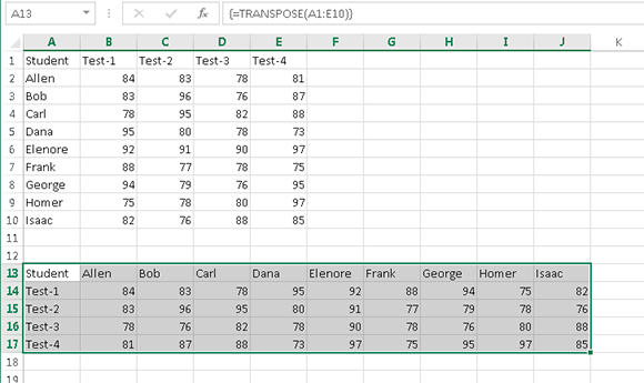
Figure 63-2:
A13:J17 contains a multicell array formula, linked to the source range.
1.
Make a note of the number of rows and columns in the source range.
In this example, the source range (A1:E10) has 10 rows and 5 columns.
2.
Select a range of blank cells that has the same number of rows as source range columns, and the same number of column as source range rows.
In this example, the selection should be 5 rows and 10 columns. For example, you can put the transposed range in A13:J17.
3.
Type a formula that uses the TRANSPOSE function, with the source range address as its argument.
In this example, the formula is
=TRANSPOSE(A1:E10)
4.
Press Ctrl+Shift+Enter (not just Enter) to create a multicell array formula in all of the selected cells.
Any changes made in the source range also appear in the transposed range.
Tip 64: Using Flash Fill to Extract Data
When you import data, it’s often necessary to clean up some of the text. For example, names may appear in uppercase that they should be in proper case. One approach is to use formulas to modify the text (see Tip 57). Another approach uses a feature introduced in Excel 2013: Flash Fill.
Flash Fill uses pattern recognition to extract data (and also concatenate data) from adjoining columns. Just enter a few examples in a column that’s adjacent to the data, and then choose Data⇒Data Tools⇒Flash Fill (or press Ctrl+E). Excel analyzes the examples you typed and attempts to fill in the remaining cells. If Excel didn’t recognize the pattern you had in mind, press Ctrl+Z, add another example or two, and try again.
Changing the case of text
Figure 64-1 shows a list of U.S. presidents in column A. Column B shows the result of using Flash Fill to convert the text to proper case.
Start by providing a few examples: Type
George Washington
in cell B1 and
John Adams
in cell B2. You’ll notice that Excel kicks in as soon as you start typing John Adams. It recognizes your pattern (which is “make all text proper case”) and fills the column with the transformed text (in a light gray color). You can press Enter to keep Excel’s suggestion, or continue typing more examples. At any time, you can press Ctrl+E to have Excel fill the column.
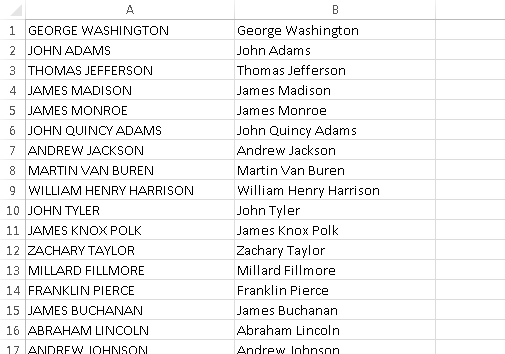
Figure 64-1:
Flash Fill quickly converted the names in Column A to proper case.
Extracting last names
In this example, we want to extract the last name of each president, so the list can be sorted by last name. This is a simple job for Flash Fill. It takes only two examples, and the pattern is recognized.
Figure 64-2 shows the worksheet after Excel extracted the last names. Now, you can sort the list by column C, so the name will be in alphabetical order, by last name.
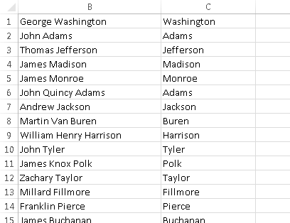
Figure 64-2:
Flash Fill extracted the last names.
Extracting first names
You’ll find that Flash Fill is equally adept at extracting first names. Figure 64-3 shows the list of presidents after using Flash Fill to extract the first names in Column D. Again, it took only two examples before Excel identified the pattern.
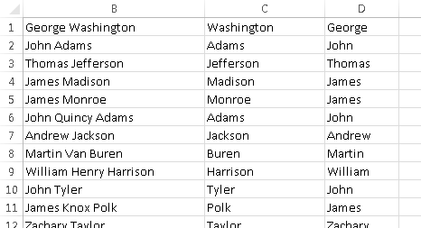
Figure 64-3:
Flash Fill extracted the first names.
Extracting middle names
Some (but not all) of the presidents on the list have a middle name. Can Flash Fill extract the middle names?
The answer: Sort of. I provided several examples of middle names, and Flash Fill successfully extracted the other middle names. But for names without a middle name, it extracted the first name. No matter what I tried, I could not get Flash Fill to ignore names that had no middle name.
Extracting domain names from URLs
Here’s another example of using Flash Fill. Say you have a list of URLs and need to extract the filename (the text that follows the last slash character).
Figure 64-4 shows a list of URLs. Flash Fill required just one example of a filename entered in column B. I pressed Ctrl+E, and Excel filled in the remaining rows. Flash fill worked equally well removing the filename from the URL, in column C.
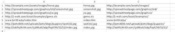
Figure 64-4:
Flash Fill extracted the filenames from URLs.
Potential problems
Flash Fill is a great feature, but if you use it for important data, you should be aware of some potential problems:
→
Sometimes it just doesn’t work.
Extracting middle names seems like a simple pattern, but Flash Fill was not capable of recognizing the pattern.
→
It’s not always accurate.
With a small set of data, it’s usually easy to check to ensure that Flash Fill worked as you intended it to work. But if you use Flash Fill on thousands of rows of data, you can’t be assured that it worked perfectly unless you examine every row. Flash Fill works best with data that is very consistent.
→
It’s not dynamic.
If you change any of the information that Flash Fill used, the changes are not reflected in the filled column.
→
There is no “audit trail.”
If you use formulas to extract data, the formulas provide documentation so anyone can figure out how the data was extracted. Using Flash Fill, on the other hand, provides no such audit trail. There is no way to see which rules Excel used to extract the data.