101 Excel 2013 Tips, Tricks and Timesavers (24 page)
Read 101 Excel 2013 Tips, Tricks and Timesavers Online
Authors: John Walkenbach

Tip 60: Finding Duplicates by Using Conditional Formatting
You might find it helpful to identify duplicate values within a range of cells. For example, take a look at Figure 60-1. Are any of the values duplicated?
One approach to identifying duplicate values is to use conditional formatting. After applying a conditional formatting rule, you can quickly spot duplicated cell values.
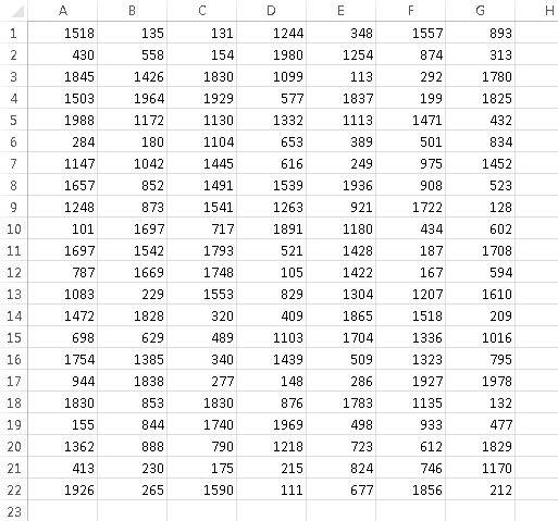
Figure 60-1:
You can use conditional formatting to quickly identify duplicate values in a range.
Here’s how to set up the conditional formatting:
1.
Select the cells in the range (in this example, A1:G22).
2.
Choose Home⇒Conditional Formatting⇒New Rule to display the Conditional Formatting dialog box.
3.
In the Conditional Formatting dialog box, select the option labeled Use a Formula to Determine Which Cells to Format.
4.
For this example, enter this formula (change the range references to correspond to your own data):
=COUNTIF($A$1:$G$22,A1)>1
5.
Click the Format button and specify the formatting to apply when the condition is true.
Changing the fill color is a good choice.
6.
Click OK.
Figure 60-2 shows the result. The seven highlighted cells are the duplicated values in the range.
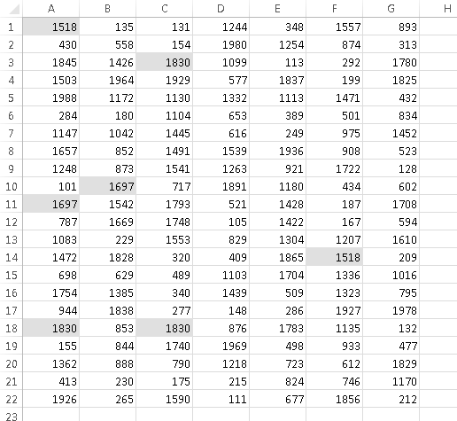
Figure 60-2:
Conditional formatting causes the duplicated cells to be highlighted.
You can extend this technique to identify entire rows within a list that are identical. The trick is to add a new column and use a formula that concatenates the data in each row. For example, if your list is in A2:G500, enter this formula in cell H2:
=A2&B2&C2&D2&E2&F2&G2
Copy the formula down the column and then apply the conditional formatting to the formulas in column H. In this case, the conditional formatting formula is
=COUNTIF($H$2:$H$500,H2)>1
Highlighted cells in column H indicate duplicated rows.
 You can use Data⇒Data Tools⇒Remove Duplicates to remove duplicate rows. That command, however, doesn’t identify the duplicates before deleting them.
Tip 61: Working with Credit Card Numbers
If you’ve ever tried to enter a 16-digit credit card number into a cell, you may have discovered that Excel always changes the last digit to a zero. Even worse, maybe you
didn’t
discover the changed credit card number until it was too late.
Why does Excel change your numbers? The reason is that Excel can handle only 15 digits of numerical accuracy.
Entering credit card numbers manually
If you need to store credit card numbers in a worksheet, you have three options:
→
Precede the credit card number with an apostrophe.
Excel then interprets the data as a text string rather than as a number.
→
Preformat the cell or range by using the Text number format.
Select the range, choose Home⇒Number and then select Text from the Number Format drop-down control.
→
Enter the card number with dashes or spaces.
Embedding a dash character (or any other non-numeric character) forces Excel to interpret the entry as text.
This tip, of course, also applies to other long numbers (such as part numbers) that aren’t used in numeric calculations.
Importing credit card numbers
If you’re importing credit card numbers from a CSV text file, Excel will import the credit card numbers as values — and erroneously change the last digit to zero. To avoid this, don’t use File⇒Open to import the text. Rather, use Data⇒Connections⇒Get External Data⇒From Text. When you use this command, Excel displays the TextImport Wizard. In Step 3 of the wizard, make sure that you specify Text as the column data format for the credit card numbers. See Figure 61-1.
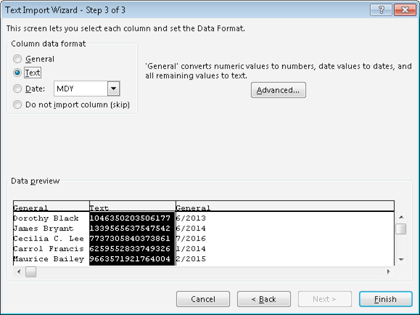
Figure 61-1:
Using the TextImport Wizard to ensure that credit card numbers are imported as text.
Tip 62: Identifying Excess Spaces
A common type of spreadsheet error involves something that you can’t even see: a space character. Consider the example shown in Figure 62-1. Cell B2 contains a formula that looks up the color name in cell B1 and returns the corresponding code from a table. The formula is
=VLOOKUP(B1,D2:E9,2,FALSE)
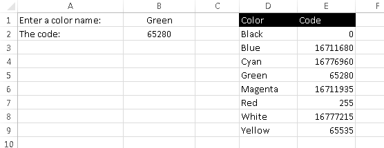
Figure 62-1:
A simple lookup formula returns the code for a color entered in cell B1.
In Figure 62-2, the formula in cell B2 returns an error — indicating that
Red
wasn’t found in the table. Hundreds of thousands of Excel users have spent far too much time trying to figure out why this sort of thing doesn’t work. In this case, the answer is simple: Cell D7 doesn’t contain the word
Red
. Rather, it contains the word
Red
followed by a space. To Excel, these text strings are completely different.

Figure 62-2:
The lookup formula can’t find the word
Red
in the table.
If your worksheet contains thousands of text entries — and you need to perform comparisons using that text — you may want to identify the cells that contain excess spaces and then fix those cells. The term
excess spaces
means a text entry that contains any of the following:
→ One or more leading spaces
→ One or more trailing spaces
→ Two or more consecutive spaces within the text
One way to identify this type of cell is to use conditional formatting. To set up conditional formatting to identify excess spaces, follow these steps:
1.
Select all text cells to which you want to apply conditional formatting.
2.
Choose Home⇒Conditional Formatting⇒New Rule to display the New Formatting Rule dialog box.
3.
In the top part of the dialog box, select the option labeled Use a Formula to Determine Which Cells to Format.
4.
Enter a formula like the following in the bottom part of the dialog box (see Figure 62-3):
=A1<>TRIM(A1)
Note:
This formula assumes that cell A1 is the upper-left cell in the selection. If that’s not the case, substitute the address of the upper-left cell in the selection you made in Step 1.
5.
Click the Format button to display the Format Cells dialog box and select the type of formatting you want for the cells that contain excess spaces — for example, a yellow fill color.
6.
Click OK to close the Format Cells dialog box, and click OK again to close the New Formatting Rule dialog box.
After you complete these steps, each cell that contains excess spaces and is within the range you selected in Step 1 is highlighted with the formatting of your choice. You can then easily spot these cells and remove the spaces.
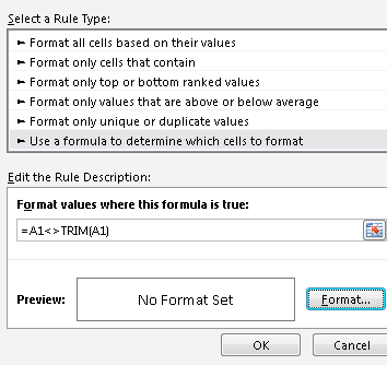
Figure 62-3:
Using conditional formatting to identify cells that contain excess spaces.
Because of the way the TRIM function works, the formula in Step 4 also applies the conditional formatting to all numeric cells. A slightly more complex formula that doesn’t apply the formatting to numeric cells is