101 Excel 2013 Tips, Tricks and Timesavers (29 page)
Read 101 Excel 2013 Tips, Tricks and Timesavers Online
Authors: John Walkenbach

Figure 72-1:
Adding the speech commands to the Ribbon.

Figure 72-2:
Speech commands added to the Ribbon.
Tip 73: Getting Data from a PDF File
A PDF file is a document format that displays text or graphics in a way that’s independent of the hardware and operating system used to create the document. PDF files are very common, and just about everyone has software that can read PDF files.
Excel can export a worksheet (or workbook) as a PDF file, but it cannot open PDF files. This tip describes two ways to get data from a PDF file into an Excel worksheet.
Using copy and paste
Figure 73-1 shows a PDF file displayed in Adobe Reader. I selected the table of data and pressed Ctrl+C to copy it to the Clipboard. Then I activated Excel and pressed Ctrl+V to copy the Clipboard contents. The result is shown in Figure 73-2.
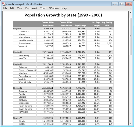
Figure 73-1:
Data in a PDF file that needs to be transferred to a worksheet.
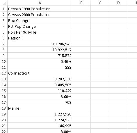
Figure 73-2:
Using copy and paste doesn’t work very well.
The data is copied, but it’s all in a single column. I could spend some time and rearrange the data, but there’s a more efficient way to transfer the PDF file data to Excel.
 When coping from a PDF file and pasting to a worksheet, the actual results will vary, depending on the layout of the PDF file. In some cases, the pasted text is usable. But in most cases, it’s not.
Using Word 2013 as an intermediary
Excel can’t open PDF files, but Word 2013 can. Figure 73-3 shows a Word document after importing the PDF file. The information can be copied and pasted to an Excel worksheet — and the result will require minimal reformatting (see Figure 73-4).
After making a few minor edits, the table looks perfect.
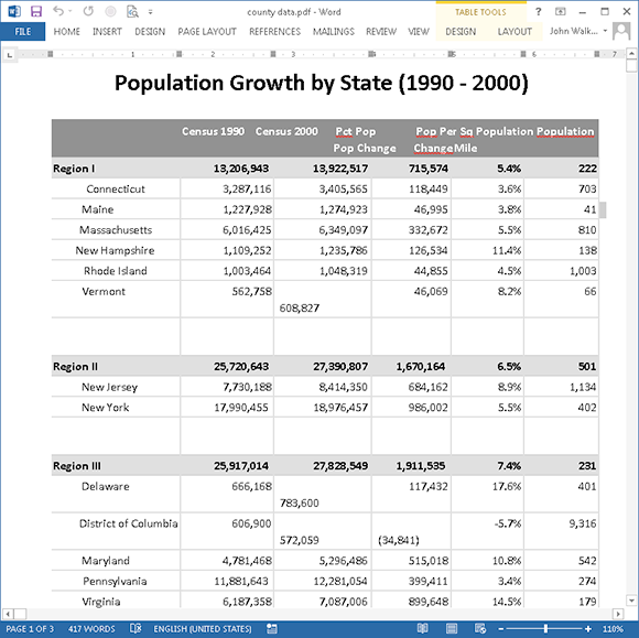
Figure 73-3:
A PDF file, imported into World 2013.
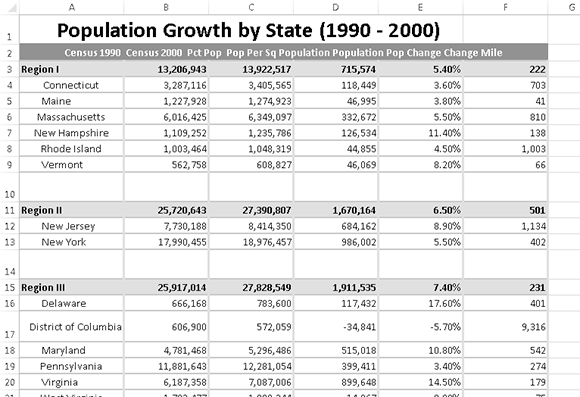
Figure 73-4:
A Word 2013 document pasted into an Excel worksheet.
The ability to open PDF files is new to Word 2013, so this method won’t work with other previous versions of Word.
Part V: Tables and Pivot Tables
This part contains tips that deal with two of Excel’s most useful features: tables and pivot tables. If you work with large amounts of structured data, you owe it to yourself to understand these features.
Tips and Where to Find Them
Tip 75:
Using Formulas with a Table
Tip 76:
Numbering Table Rows Automatically
Tip 77:
Identifying Data Appropriate for a Pivot Table
Tip 78:
Using a Pivot Table Instead of Formulas
Tip 79:
Controlling References to Cells Within a Pivot Table
Tip 80:
Creating a Quick Frequency Tabulation
Tip 81:
Grouping Items by Date in a Pivot Table
Tip 74: Understanding Tables
An important but often underutilized feature in Excel is tables. This tip describes when to use a table and also lists the advantages and disadvantages.
Understanding what a table is
A
table
is a rectangular range of structured data. Each row in the table corresponds to a single entity. For example, a row can contain information about a customer, a bank transaction, an employee, or a product. Each column contains a specific piece of information. For example, if each row contains information about an employee, the columns can contain data, such as name, employee number, hire date, salary, or department. Tables have a header row at the top that describes the information contained in each column.
You’ve probably created ranges that meet this description. The magic happens when you tell Excel to convert a range of data into an “official” table. You do so by selecting any cell within the range and then choosing Insert⇒Tables⇒Table.
When you explicitly identify a range as a table, Excel can respond more intelligently to the actions you perform with that range. For example, if you create a chart from a table, the chart expands automatically as you add new rows to the table. If you create a pivot table from a table, refreshing the pivot table will include any new data that you added to the table.
Figure 74-1 shows a range before it was converted to a table, and Figure 74-2 shows the range after it was converted to a table.
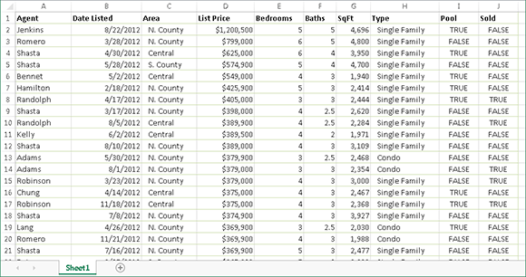
Figure 74-1:
A range of data that’s not an official table.

Figure 74-2:
A range of data that has been designated a table.
Range versus table
What’s the difference between a standard range and a range that has been converted to a table?
→ Activating any cell in the table gives you access to a new Table Tools context tab on the Ribbon.
→ You can quickly apply background color and text color formatting by choosing from a gallery. This type of formatting is optional.
→ Each column header contains a filter button that, when clicked, lets you easily sort the rows or filter the data by hiding rows that don’t meet your criteria.
→ A table can have “slicers,” which makes it easy for novices to quickly apply filters to a table.
→ If you scroll down the sheet so that the header row disappears, the table headers replace the column letters in the worksheet header. In other words, you don’t need to freeze the top row to keep the column labels visible.
→ If you create a chart from data in a table, the chart automatically expands if you add new rows to the end of the table.
→ If you create a name for a column in a table, the “refers to” range for the name adjusts as you add new rows to the table.
→ Tables support calculated columns. A single formula entered in a cell is automatically propagated to all cells in the column (see Tip 75).
→ Tables support structured references in formulas outside of the table. Rather than use cell references, formulas can use table names and column headers.
→ When you move your mouse pointer to the lower-right corner of the lower-right cell, you can click and drag to extend the table’s size, either horizontally (add more columns) or vertically (add more rows).
→ Selecting rows and columns within the table is simplified.
Limitations of using a table
If a workbook contains at least one table, a few Excel features are not available:
→ For some reason, when a workbook contains at least one table, Excel doesn’t allow you to use the Custom Views feature (choose View⇒Workbook Views⇒Custom Views).
→ You cannot share a workbook (using Review⇒Changes⇒Share) if the workbook contains a table.
→ You can’t insert automatic subtotals within a table (by choosing Data⇒Outline⇒Subtotal).
→ You cannot use array formulas within a table.
Tip 75: Using Formulas with a Table
This tip describes some ways to use formulas with a table. The example uses a simple sales summary table with three columns: Month, Projected, and Actual, as shown in Figure 75-1. I entered the data and then converted the range to a table by using the Insert⇒Tables⇒Table command. Note that I didn’t define any names, but the data area of the table is named Table1 by default.
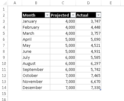
Figure 75-1:
A simple table with three columns.
Working with the Total row
If you want to calculate the total projected and total actual sales, you don’t even need to write a formula. Just click a button to add a row of summary formulas to the table:
1.
Activate any cell in the table.
2.
Select the Table Tools⇒Design⇒Table Style Options⇒Total Row command and check the Total Row check box.
3.
Activate a cell in the Total row and select a summary formula from the drop-down list (see Figure 75-2).
For example, to calculate the sum of the Actual column, select SUM from the drop-down list in cell D15. Excel creates this formula:
=SUBTOTAL(109,[Actual])
For the SUBTOTAL function, 109 is an enumerated argument that represents SUM. The second argument for the SUBTOTAL function is the column name, in square brackets. Using the column name within brackets is a way to create structured references within a table.

Figure 75-2:
A drop-down list enables you to select a summary formula for a table column.
You can toggle the Total row display on and off by choosing Table Tools⇒Design
➜
Table Style Options⇒Total Row. If you turn it off, the summary options you selected are remembered when you turn it back on.
Using formulas within a table
In many cases, you want to use formulas within a table. For example, in the table shown in Figure 75-1, you may want a column that shows the difference between the actual and projected amounts for each month. As you can see, Excel makes this process very easy:
1.
Activate cell E2 and type
Difference
for the column header.
Excel automatically expands the table for you.
2.
Move to cell E3 and type an equal sign (
=
) to signal the beginning of a formula.
3.
Press the left-arrow key to point to the corresponding value in the Actual column.
4.
Type a minus sign (
–
) and then press the left-arrow key twice to point to the corresponding value in the Projected column.
5.
Press Enter to end the formula.
The formula is entered into the other cells in the column, and the Formula bar displays this formula:
=[@Actual]-[@Projected]
Figure 75-3 shows the table with the new column.
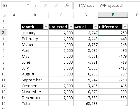
Figure 75-3:
The Difference column contains a formula.
Although the formula was entered into the first row of the table, that’s not necessary. Anytime a formula is entered into an empty table column, it propagates to the other cells in the column. If you need to edit the formula, edit any formula in the column, and the change is applied to the other cells in the column.
Propagating a formula to other cells in a table column is actually one of Excel’s AutoCorrect options. To turn off this feature, click the icon that appears when you enter a formula and choose Stop Automatically Creating Calculated Columns.