Programming Python (183 page)

Many problems
that crop up in both real life and real programming can be
fairly represented as a graph—a set of states with transitions (“arcs”)
that lead from one state to another. For example, planning a route for a
trip is really a graph search problem in disguise: the states are places
you’d like to visit, and the arcs are the transportation links between
them. A program that searches for a trip’s optimal route is a graph
searcher. For that matter, so are many programs that walk hyperlinks on
the Web.
This section presents simple Python programs that search through a
directed, cyclic graph to find the paths between a start state and a goal.
Graphs can be more general than trees because links may point at arbitrary
nodes—even ones already searched (hence the word
cyclic
). Moreover, there isn’t any direct built-in
support for this type of goal; although graph searchers may ultimately use
built-in types, their search routines are custom enough to warrant
proprietary implementations.
The graph used to test searchers in this section is sketched in
Figure 18-1
. Arrows at the end of arcs indicate
valid paths (e.g.,
A
leads to
B,
E
, and
G
). The search algorithms will
traverse this graph in a depth-first fashion, and they will trap cycles in
order to avoid looping. If you pretend that this is a map, where nodes
represent cities and arcs represent roads, this example will probably seem
a bit more meaningful.
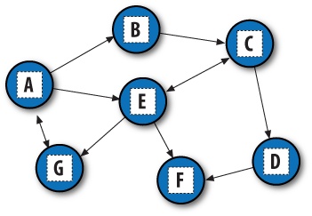
Figure 18-1. A directed graph
The first thing
we need to do is choose a way to represent this graph in a
Python script. One approach is to use built-in datatypes and searcher
functions. The file in
Example 18-16
builds the test
graph as a simple dictionary: each state is a dictionary key, with a
list of keys of nodes it leads to (i.e., its arcs). This file also
defines a function that we’ll use to run a few searches in the
graph.
Example 18-16. PP4E\Dstruct\Classics\gtestfunc.py
"dictionary based graph representation"
Graph = {'A':  ['B', 'E', 'G'],
'B':  ['C'],                        # a directed, cyclic graph
'C':  ['D', 'E'],                   # stored as a dictionary
'D':  ['F'],                        # 'key' leads-to [nodes]
'E':  ['C', 'F', 'G'],
'F':  [ ],
'G':  ['A']  }
def tests(searcher):                         # test searcher function
print(searcher('E', 'D', Graph))         # find all paths from 'E' to 'D'
for x in ['AG', 'GF', 'BA', 'DA']:
print(x, searcher(x[0], x[1], Graph))
Now, let’s code two modules that implement the actual search
algorithms. They are both independent of the graph to be searched (it is
passed in as an argument). The first searcher, in
Example 18-17
, uses
recursion
to walk through the graph.
Example 18-17. PP4E\Dstruct\Classics\gsearch1.py
"find all paths from start to goal in graph"
def search(start, goal, graph):
solns = []
generate([start], goal, solns, graph)              # collect paths
solns.sort(key=lambda x: len(x))                   # sort by path length
return solns
def generate(path, goal, solns, graph):
state = path[-1]
if state == goal:                                  # found goal here
solns.append(path)                             # change solns in-place
else:                                              # check all arcs here
for arc in graph[state]:                       # skip cycles on path
if arc not in path:
generate(path + [arc], goal, solns, graph)
if __name__ == '__main__':
import gtestfunc
gtestfunc.tests(search)
The second searcher, in
Example 18-18
, uses an explicit
stack
of paths to be expanded using the tuple-tree
stack representation we explored earlier in this chapter.
Example 18-18. PP4E\Dstruct\Classics\gsearch2.py
"graph search, using paths stack instead of recursion"
def search(start, goal, graph):
solns = generate(([start], []), goal, graph)
solns.sort(key=lambda x: len(x))
return solns
def generate(paths, goal, graph):                      # returns solns list
solns = []                                         # use a tuple-stack
while paths:
front, paths = paths                           # pop the top path
state = front[-1]
if state == goal:
solns.append(front)                        # goal on this path
else:
for arc in graph[state]:                   # add all extensions
if arc not in front:
paths = (front + [arc]), paths
return solns
if __name__ == '__main__':
import gtestfunc
gtestfunc.tests(search)
To avoid cycles, both searchers keep track of nodes visited along
a path. If an extension is already on the current path, it is a loop.
The resulting solutions list is sorted by increasing lengths using the
listsortmethod and its optionalkeyvalue transform argument. To test
the searcher modules, simply run them; their self-test code calls the
canned search test in thegtestfuncmodule:
C:\...\PP4E\Dstruct\Classics>python gsearch1.py[['E', 'C', 'D'], ['E', 'G', 'A', 'B', 'C', 'D']]
AG [['A', 'G'], ['A', 'E', 'G'], ['A', 'B', 'C', 'E', 'G']]
GF [['G', 'A', 'E', 'F'], ['G', 'A', 'B', 'C', 'D', 'F'],
['G', 'A', 'B', 'C', 'E', 'F'], ['G', 'A', 'E', 'C', 'D', 'F']]
BA [['B', 'C', 'E', 'G', 'A']]
DA []
C:\...\PP4E\Dstruct\Classics>python gsearch2.py[['E', 'C', 'D'], ['E', 'G', 'A', 'B', 'C', 'D']]
AG [['A', 'G'], ['A', 'E', 'G'], ['A', 'B', 'C', 'E', 'G']]
GF [['G', 'A', 'E', 'F'], ['G', 'A', 'E', 'C', 'D', 'F'],
['G', 'A', 'B', 'C', 'E', 'F'], ['G', 'A', 'B', 'C', 'D', 'F']]
BA [['B', 'C', 'E', 'G', 'A']]
DA []
This output shows lists of possible paths through the test graph;
I added two line breaks to make it more readable (Pythonpprintpretty-printer module might help with
readability here as well). Notice that both searchers find the same
paths in all tests, but the order in which they find those solutions may
differ. Thegsearch2order depends on
how and when extensions are added to its path’s stack; try tracing
through the outputs and code to see
how.
Using dictionaries to
represent graphs is efficient: connected nodes are located
by a fast hashing operation. But depending on the application, other
representations might make more sense. For instance, classes can be used
to model nodes in a network, too, much like the binary tree example
earlier. As classes, nodes may contain content useful for more
sophisticated searches. They may also participate in inheritance
hierarchies, to acquire additional behaviors. To illustrate the basic
idea,
Example 18-19
shows an
alternative coding for our graph searcher; its algorithm is closest togsearch1.
Example 18-19. PP4E\Dstruct\Classics\graph.py
"build graph with objects that know how to search"
class Graph:
def __init__(self, label, extra=None):
self.name = label                                # nodes=inst objects
self.data = extra                                # graph=linked objs
self.arcs = []
def __repr__(self):
return self.name
def search(self, goal):
Graph.solns = []
self.generate([self], goal)
Graph.solns.sort(key=lambda x: len(x))
return Graph.solns
def generate(self, path, goal):
if self == goal:                                 # class == tests addr
Graph.solns.append(path)                     # or self.solns: same
else:
for arc in self.arcs:
if arc not in path:
arc.generate(path + [arc], goal)
In this version, graphs are represented as a network of embedded
class instance objects. Each node in the graph contains a list of the
node objects it leads to (arcs),
which it knows how to search. Thegeneratemethod walks through the objects in
the graph. But this time, links are directly available on each node’sarcslist; there is no need to index
(or pass) a dictionary to find linked objects. The search is effectively
spread across the graph’s linked objects.
To test, the module in
Example 18-20
builds the test
graph again, this time using linked instances of theGraphclass. Notice the use ofexecin this code: it executes dynamically
constructed strings to do the work of seven assignment statements
(A=Graph('A'),B=Graph('B'), and so on).
Example 18-20. PP4E\Dstruct\Classics\gtestobj1.py
"build class-based graph and run test searches"
from graph import Graph
# this doesn't work inside def in 3.1: B undefined
for name in "ABCDEFG":                               # make objects first
exec("%s = Graph('%s')" % (name, name))          # label=variable-name
A.arcs = [B, E, G]
B.arcs = [C]                 # now configure their links:
C.arcs = [D, E]              # embedded class-instance list
D.arcs = [F]
E.arcs = [C, F, G]
G.arcs = [A]
A.search(G)
for (start, stop) in [(E,D), (A,G), (G,F), (B,A), (D,A)]:
print(start.search(stop))
Running this test executes the same sort of graph walking, but
this time it’s routed through object methods:
C:\...\PP4E\Dstruct\Classics>python gtestobj1.py[[E, C, D], [E, G, A, B, C, D]]
[[A, G], [A, E, G], [A, B, C, E, G]]
[[G, A, E, F], [G, A, B, C, D, F], [G, A, B, C, E, F], [G, A, E, C, D, F]]
[[B, C, E, G, A]]
[]
The results are the same as for the functions, but node name
labels are not quoted: nodes on path lists here areGraphinstances, and this class’s__repr__scheme suppresses quotes.
Example 18-21
is one last graph
test before we move on; sketch the nodes and arcs on paper if you have
more trouble following the paths than Python.
Example 18-21. PP4E\Dstruct\Classics\gtestobj2.py
from graph import Graph
S = Graph('s')
P = Graph('p')       # a graph of spam
A = Graph('a')       # make node objects
M = Graph('m')
S.arcs = [P, M]      # S leads to P and M
P.arcs = [S, M, A]   # arcs: embedded objects
A.arcs = [M]
print(S.search(M))   # find all paths from S to M
This test finds three paths in its graph between nodes S and M.
We’ve really only scratched the surface of this academic yet useful
domain here; experiment further on your own, and see other books for
additional topics (e.g.,
breadth-first
search by
levels, and
best-first
search by path or state
scores):
C:\...\PP4E\Dstruct\Classics>python gtestobj2.py[[s, m], [s, p, m], [s, p, a, m]]
Our next data
structure topic implements extended functionality for
sequences that is not present in Python’s built-in objects. The functions
defined in
Example 18-22
shuffle sequences in a number of ways:
permuteconstructs a list with all valid permutations of any
sequencesubsetconstructs a list with all valid permutations of a specific
lengthcomboworks like
subset, but
order doesn’t matter: permutations of the same items are filtered
out
These results are useful in a variety of algorithms: searches,
statistical analysis, and more. For instance, one way to find an optimal
ordering for items is to put them in a list, generate all possible
permutations, and simply test each one in turn. All three of the functions
make use of generic sequence slicing so that the result list contains
sequences of the same type as the one passed in (e.g., when we permute a
string, we get back a list of strings).
Example 18-22. PP4E\Dstruct\Classics\permcomb.py
"permutation-type operations for sequences"
def permute(list):
if not list:                                        # shuffle any sequence
return [list]                                   # empty sequence
else:
res = []
for i in range(len(list)):
rest = list[:i] + list[i+1:]                # delete current node
for x in permute(rest):                     # permute the others
res.append(list[i:i+1] + x)             # add node at front
return res
def subset(list, size):
if size == 0 or not list:                            # order matters here
return [list[:0]]                                # an empty sequence
else:
result = []
for i in range(len(list)):
pick = list[i:i+1]                           # sequence slice
rest = list[:i] + list[i+1:]                 # keep [:i] part
for x in subset(rest, size-1):
result.append(pick + x)
return result
def combo(list, size):
if size == 0 or not list:                            # order doesn't matter
return [list[:0]]                                # xyz == yzx
else:
result = []
for i in range(0, (len(list) - size) + 1):       # iff enough left
pick = list[i:i+1]
rest = list[i+1:]                            # drop [:i] part
for x in combo(rest, size - 1):
result.append(pick + x)
return result
All three of these functions work on any sequence object that
supportslen, slicing, and
concatenation operations. For instance, we can usepermuteon instances of some of the stack
classes defined at the start of this chapter (experiment with this on your
own for more insights).
The following session shows our sequence shufflers in action.
Permuting a list enables us to find all the ways the items can be
arranged. For instance, for a four-item list, there are 24 possible
permutations (4 × 3 × 2 × 1). After picking one of the four for the first
position, there are only three left to choose from for the second, and so
on. Order matters:[1,2,3]is not the
same as[1,3,2], so both appear in the
result:
C:\...\PP4E\Dstruct\Classics>python>>>from permcomb import *>>>permute([1, 2, 3])[[1, 2, 3], [1, 3, 2], [2, 1, 3], [2, 3, 1], [3, 1, 2], [3, 2, 1]]
>>>permute('abc')['abc', 'acb', 'bac', 'bca', 'cab', 'cba']
>>>permute('help')['help', 'hepl', 'hlep', 'hlpe', 'hpel', 'hple', 'ehlp', 'ehpl', 'elhp', 'elph',
'ephl', 'eplh', 'lhep', 'lhpe', 'lehp', 'leph', 'lphe', 'lpeh', 'phel', 'phle',
'pehl', 'pelh', 'plhe', 'pleh']
comboresults are related to
permutations, but a fixed-length constraint is put on the result, and
order doesn’t matter:abcis the same
asacb, so only one is added to the
result set:
>>>combo([1, 2, 3], 3)[[1, 2, 3]]
>>>combo('abc', 3)['abc']
>>>combo('abc', 2)['ab', 'ac', 'bc']
>>>combo('abc', 4)[]
>>>combo((1, 2, 3, 4), 3)[(1, 2, 3), (1, 2, 4), (1, 3, 4), (2, 3, 4)]
>>>for i in range(0, 6): print(i, combo("help", i))...
0 ['']
1 ['h', 'e', 'l', 'p']
2 ['he', 'hl', 'hp', 'el', 'ep', 'lp']
3 ['hel', 'hep', 'hlp', 'elp']
4 ['help']
5 []
Finally,subsetis just
fixed-length permutations; order matters, so the result is larger than forcombo. In fact, callingsubsetwith the length of the sequence is
identical topermute:
>>>subset([1, 2, 3], 3)[[1, 2, 3], [1, 3, 2], [2, 1, 3], [2, 3, 1], [3, 1, 2], [3, 2, 1]]
>>>subset('abc', 3)['abc', 'acb', 'bac', 'bca', 'cab', 'cba']
>>>for i in range(0, 6): print(i, subset("help", i))...
0 ['']
1 ['h', 'e', 'l', 'p']
2 ['he', 'hl', 'hp', 'eh', 'el', 'ep', 'lh', 'le', 'lp', 'ph', 'pe', 'pl']
3 ['hel', 'hep', 'hle', 'hlp', 'hpe', 'hpl', 'ehl', 'ehp', 'elh', 'elp', 'eph',
'epl', 'lhe', 'lhp', 'leh', 'lep', 'lph', 'lpe', 'phe', 'phl', 'peh', 'pel',
'plh', 'ple']
4 ['help', 'hepl', 'hlep', 'hlpe', 'hpel', 'hple', 'ehlp', 'ehpl', 'elhp',
'elph', 'ephl', 'eplh', 'lhep', 'lhpe', 'lehp', 'leph', 'lphe', 'lpeh',
'phel', 'phle', 'pehl', 'pelh', 'plhe', 'pleh']
5 ['help', 'hepl', 'hlep', 'hlpe', 'hpel', 'hple', 'ehlp', 'ehpl', 'elhp',
'elph', 'ephl', 'eplh', 'lhep', 'lhpe', 'lehp', 'leph', 'lphe', 'lpeh',
'phel', 'phle', 'pehl', 'pelh', 'plhe', 'pleh']
These are some fairly dense algorithms (and frankly, may seem to
require a Zen-like “moment of clarity” to grasp completely), but they are
not too obscure if you trace through a few simple cases first. They’re
also representative of the sort of operation that requires custom data
structure code—unlike the last stop on our data structures tour in the
next section.