More Guns Less Crime (29 page)
Read More Guns Less Crime Online
Authors: John R. Lott Jr
Tags: #gun control; second amendment; guns; crime; violence

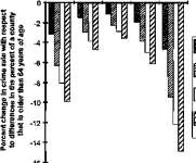
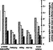
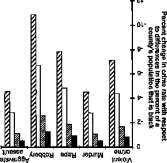
The results reported in figures 9.6—9.9 are all quite statistically significant and imply the same pattern reported earlier when using the data through 1992. The benefits of right-to-carry laws are not uniform across counties. Counties with a high portion of elderly people, blacks, and females—the most vulnerable victims—all benefit disproportionately more from concealed-handgun laws. So do those living in counties that are densely populated.
Certain crime patterns do emerge. For example, in counties with many elderly people (23 percent of the population over age sixty-four) right-to-carry laws have a large deterrent effect against aggravated assaults and robberies but seem to have a relatively small effect on rapes. In contrast, counties with few elderly individuals (7 percent of their population over sixty-four years of age) have only about a third of the drop in violent crime that counties with many elderly people have. Heavily black areas benefit the most through reductions in robberies and rapes, while areas where women make up a larger share of the population and those living in the wealthiest areas obtain the largest benefits from drops in aggravated assaults and rapes. The benefit for blacks is very large. Increasing the percentage of the black population in a county from half the mean (4.4 percent) to two standard deviations above the mean (37 per-
Violent _ _ .. .. BS ,.-.—.
crime Murder Rape Robbery assauil

B1/2 Mean population that is over 64 years old (0.071535)
i Mean population that is over 64 jyearsold(0.14307)
iMean population that is over 64 years old plus one standard J deviation (0.1842)
J Mean population that is over 64 j years old plus two standard deviations (0.2254)
Violent-crime categories
Figure 9.6. How does the change in crime from nondiscretionary concealed-handgun laws occur in counties with relatively more people over age sixty-four?
lj li fl
n it
it
£8
U
u
0 -0.5
-1 -1.5
-2 -2.5
-3 -3.5
-4 -4.5
Violent crime
Murder
BUL Aggravated Rape Robbery a8Sauit
11/2 Mean population density per square mile (82)
J Mean population density per 3 square mile (163.9)
1 Mean population density per square mile plus one standard deviation (703)
i Mean population density per ] square mile plus two standard deviations (1242)
Violent-crime categories
Figure 9.7. How does the change in crime from nondiscretionary concealed-handgun laws occur in the most densely populated counties?
cent) increases the reduction in violent crime from right-to-carry laws from about one percentage point to over seven percentage points.
Unlike the earlier data presented in chapter 4, which represented crime through 1992, not all the states adopting right-to-carry laws during 1993—1996 moved from a discretionary to a nondiscretionary law Some states had previously prohibited the carrying of concealed handguns. This is important because one of the reasons that I examined the interactions of population or population density with right-to-carry laws was that state government officials had told me that under a discretionary system lower-population counties had already tended to be more liberal
(sB3xe ireqm ui Suiaij asoqj pire s^DBjq) suilpia auiiio aq o* Xp^ij jsoui a.re oqA\ asoqi ptre (Ajiapp aqi pui> U3uioa\) AjpDisAqd J3^3M XpAij^pi 3i^ oqA\ asoqi jizqi s8uipuu laqiiza Aui uiiuuod s:qns3i pa^pdn asaqx
•SA\iq AjiziiopaiDsipiioii oi sunSpireq p3p33UOD 8uiuireq uiojj paSireqD jisqi saji^s ireqj szxvi auiiiD-juajoiA ui doip 3Ai?epj J388iq XipgDiisims ^ p^q SA\iq AxeuonaiDsipuou oi XxeuouaiD -sip uiojj 8ui8ueq3 saigas ui sauunco sncqndod aioui aqj reqi puu j ':pi2j uj paidopis si»a\ uiaisAs AxeuonaiDsipuou 12 jrajjB auiiio juajoiA ui sdojp IsaSxej aqj snqj pue sjiuiiad 8uinssi ui araaiDui isaSxej aqj 33U3U3dx3 oi p3i33dx3 snqj 3J3a\ sanunco uoniqndod-iaqSijj # siiuiJ3d SuiiireiS ui
^auiODui BjidBD-iad A^urtoD qjiA\ Xiba sa\bj un2puBq-p3[B33UOD AiBuoiaaiDsipuou uiojj 3UIIJD ui aSuBqD aqa saop A\ofj '6'6 3Jn ^H
(W€'9l$) suorbjabp pjepuB)6 n om) snjd eiuooui eudeo-jsd ubsw Q
(Z8Z'Ct$) U0JJBIA9P pjBpUB^ n
euo enjd ouiooui eydeo-jed ueow U
eiuoou] eudeo-jad ubs^H
(S09'S$)|
oiuoou! eiideo-jed ueeft Zll *

pS,^
^DB|q si jBqi uonBjrtdod s ( A^urto3 b jo axfejuaDiad aqi qjiA\ Xjba sa\b| un2puBq-pa|B3DUOD XiBuopaiDsipuou uiojj 3UIU3 ui aSuBqD aqi saop A\opj g^ airtSij
sejjoBoieo euijj>iuo|0|A
(Z'ZC) 8UORB|A9p PJBPU8)6 OM)
snjd jpsjq si jBifl uogBindod ubow Q
(CZ) uoRBiAep pjBpueje euo sn|d )psiq s\ jeifl uogeindod ueew |J
(88) >p8|q 8] jeifl uoRBindod ueeyy
>pB|q si ibuj uoiVBindod useifl Z/l I

p*E&/*WW edm »p« W
£8T /anooiua
tend to benefit the most from the passage of right-to-carry laws. Taken together, these results indicate that legislators should be sensitive not only to the costs of running the permitting program, but also to how the rules affect the number and types of people who get permits. Focusing only on setting fees to recoup the costs of the permitting system will end up being financially short sighted.
How Sensitive Are the Results to Different Specifications?
While I have tried to control for all sorts of factors that might explain changes in crime over time, it is indeed possible to get overzealous and account for too many variables. Including variables that do not really affect crime can actually create problems similar to excluding factors that should be included. Take a simple example of explaining how the stock market, say the Dow Jones industrials, changes over time. Obvious variables to include would be the interest rate and the expected growth in the economy, but many other variables—many of dubious importance— could possibly also be included. The problem arises when such variables are correlated to changes in stock prices merely by chance. An extreme case would be including the prices of various grocery store products. A store might sell thousands of items, and one—say, the price of peanut butter—might happen to be highly correlated with the stock prices over the particular period examined. We know that peanut butter has little to do with explaining overall stock prices, but if it just accidentally happens to move up and down with the movements in the stock market, other variables (like the interest rate) may no longer prove to be statistically significant.
There are ways to protect against this "dubious variable" problem. One is to expand the sample period. If no true causal relationship exists between the two variables, the probability that this coincidence will continue to occur during future years is low. And this is exactly what I have done as more data have become available: first by looking at data through 1992, then extending them to 1994, and now up until 1996. Another approach guarding against the "dubious variable" problem is to replicate the same test in many different places. Again, this is exactly what I have done here: I have studied the impact of right-to-carry laws in different states at different times. As charged by many a critic, it is still conceivable that some other factor just happened to occur also when an individual state passed the law, but the probability of mere coincidence falls as the experiences of more and more states are examined. It is also possible that
EPILOGUE/ 185
adding variables that don't belong can cause you to get a more significant result for other factors than is warranted.
Generally, excluding variables that should be included is a more significant problem than including variables that should not be included, and in general I have tried to err on the side of including whatever possible factors can be included. Indeed, a strong case can be made that one must be careful not to include too many variables like state time trends, which can be endlessly added on and have little theoretical justification. Still, I do not consider any of these variables to be similar to the price of peanut butter at the local grocery store in the previous discussion, but obviously some researchers might believe that some variables should not be included. One way to investigate this issue is to include only those variables that different investigators view as relevant. In the early stages of my research, when I presented my original research as a working paper at seminars, I asked participants for other factors that should be included, and some of their comments were very helpful. I also tried in vain to ask pro-gun-control researchers what variables they wanted me to include in the regressions, but (as discussed in chapter 7) they did not make any suggestions when my initial research was circulated for comments. What comments they made after the publicity broke claimed that I had not controlled for factors that I had indeed accounted for.
Since the original research immediately received a lot of attention, I have let my critics decide for themselves what variables should be included by simply giving them complete access to the data. I know from personal communication that some critics (such as Black and Nagin) did indeed examine numerous different specifications. 21
A more systematic, if time-consuming, approach is to try all possible combinations of these so-called control variables—factors which may be interesting but are included so that we can be sure of the importance of some other "focus" variables. 22 In my regressions to explain crime rates there are at least nine groups of control variables—population density, waiting periods and background checks, penalties for using guns in the commission of a crime, per-capita income, per-capita unemployment insurance payments, per-capita income maintenance payments, retirement payments per person for those over sixty-five, state poverty rate, and state unemployment rate. 23 To run all possible combinations of these nine groups of control variables requires 512 regressions. The regressions for murder rates also require a tenth control variable for the death-penalty execution rate and thus results in 1,024 combinations of control variables. Given the nine different crime categories, this amounts to 5,120 regressions.
This approach is decidedly biased toward not finding a consistent effect of the right-to-carry laws, because it includes many combinations of control variables that no researcher thinks are correct specifications. Indeed, even the strongest, best-accepted empirical relationships usually fail this test. 24 Since different people will have different preferences for what variables should be included, this massive set of results makes sense only if one knows what variables produce what results. If a range of conflicting estimates are then produced, people can judge for themselves what they think the "true" range of the estimates is.
Two sets of variables have been primarily used to test the impact of right-to-carry laws: crime trends before and after the adoption of right-to-carry laws and the percentage of people with permits. Yet another division is possible by focusing on counties with a large number of people to avoid the difficulty that low-population counties frequently have zero murder or rape rates and thus have "undefined" arrest rates. 25 Eliminating counties with fewer than 20,000 people removes about 70 percent of the missing arrest ratios for murder while sacrificing 20 percent of the observations (the population-weighted frequencies are 23 and 6 percent, respectively). Dropping out more populous counties reduces the sample size but has virtually no impact on further reducing the frequency of missing arrest rates. Even if I limit the estimates to the full sample and counties with more than 20,000 people, combining that with the two other types of specifications now results in 20,480 regressions. Because of all the concerns over possible crime trends, all estimates include variables to account for the average differences across counties and years as well as by year within region as well as the thirty-six demographic variables. 26