The Bell Curve: Intelligence and Class Structure in American Life (10 page)

The same process occurred around the country, as the figure below shows. We picked out colleges with freshman SAT-Verbal means that were separated by roughly fifty-point intervals as of 1961.
¹⁵
The specific schools named are representative of those clustering near each break point. At the bottom is a state college in the second echelon of a state system (represented by Georgia Southern); then comes a large state university (North Carolina State), then five successively more selective private schools: Villanova, Tulane, Colby, Amherst, and Harvard. We have placed the SAT scores against the backdrop of the overall distribution of SAT scores for the entire population of high school seniors (not just those who ordinarily take the SAT), using a special study that the College Board conducted in the fall of 1960. The figure points to the general phenomenon already noted for Harvard: By 1961, a large
gap separated the student bodies of the elite schools from those of the public universities. Within the elite schools, another and significant level of stratification had also developed.

Cognitive stratification in colleges by 1961

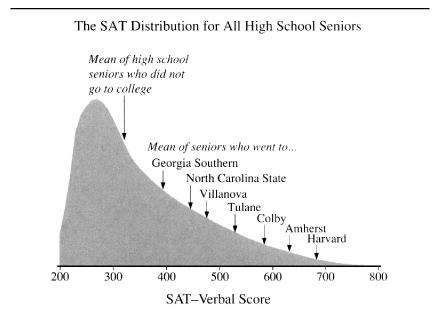
Source:
Seibel 1962; College Entrance Examination Board 1961.

As the story about Harvard indicated, the period of this stratification seems to have been quite concentrated, beginning in the early 1950s.
¹⁶
It remains to explain why. What led the nation’s most able college age youth (and their parents) to begin deciding so abruptly that State U. was no longer good enough and that they should strike out for New Haven or Palo Alto instead?

If the word
democracy
springs to your tongue, note that democracy—at least in the economic sense—had little to do with it. The Harvard freshman class of 1960 comprised fewer children from low-income families, not more, than the freshman class in 1952.
¹⁷
And no wonder. Harvard in 1950 had been cheap by today’s standards. In 1950, total costs for a year at Harvard were only $8,800—in 1990 dollars, parents of today’s college students will be saddened to learn. By 1960, total costs there had risen to $12,200 in 1990 dollars, a hefty 40 percent increase. According to the guidelines of the times, the average family could, if it
stretched, afford to spend 20 percent of its income to send a child to Harvard.
¹⁸
Seen in that light, the proportion of families who could afford Harvard
decreased
slightly during the 1950s.
¹⁹
Scholarship help increased but not fast enough to keep pace.

Nor had Harvard suddenly decided to maximize the test scores of its entering class. In a small irony of history, the Harvard faculty had decided in 1960
not
to admit students purely on the basis of academic potential as measured by tests but to consider a broader range of human qualities.
²⁰
Dean Bender explained why, voicing his fears that Harvard would “become such an intellectual hot-house that the unfortunate aspects of a self-conscious ‘intellectualism’ would become dominant and the precious, the brittle and the neurotic take over.” He asked a very good question indeed: “In other words, would being part of a super-elite in a high prestige institution be good for the healthy development of the ablest 18- to 22-year-olds, or would it tend to be a warping and narrowing experience?”
²¹
In any case, Harvard in 1960 continued, as it had in the past and would in the future, to give weight to such factors as the applicant’s legacy (was the father a Harvard alum?), his potential as a quarterback or stroke for the eight-man shell, and other nonacademic qualities.
²²

The baby boom had nothing to do with the change. The leading edge of the baby boomer tidal wave was just beginning to reach the campus by 1960.
²³

So what had happened? With the advantage of thirty additional years of hindsight, two trends stand out more clearly than they did in 1960.

First, the 1950s were the years in which television came of age and long-distance travel became commonplace. Their effects on the attitudes toward college choices can only be estimated, but they were surely significant. For students coming East from the Midwest and West, the growth of air travel and the interstate highway system made travel to school faster for affluent families and cheaper for less affluent ones. Other effects may have reflected the decreased psychic distance of Boston from parents and prospective students living in Chicago or Salt Lake City, because of the ways in which the world had become electronically smaller.

Second, the 1950s saw the early stages of an increased demand that results not from proportional changes in wealth but from an expanding number of affluent customers competing for scarce goods. Price increases for a wide variety of elite goods have outstripped changes in the
consumer price index or changes in mean income in recent decades, sometimes by orders of magnitude. The cost of Fifth Avenue apartments, seashore property, Van Gogh paintings, and rare stamps are all examples. Prices have risen because demand has increased and supply cannot. In the case of education, new universities are built, but not new Princetons, Harvards, Yales, or Stanfords. And though the proportion of families with incomes sufficient to pay for a Harvard education did not increase significantly during the 1950s, the raw number did. Using the 20-percent-of-family-income rule, the number of families that could afford Harvard increased by 184,000 from 1950 to 1960. Using a 10 percent rule, the number increased by 55,000. Only a small portion of these new families had children applying to college, but the number of slots in the freshmen classes of the elite schools was also small. College enrollment increased from 2.1 million students in 1952 to 2.6 million by 1960, meaning a half-million more competitors for available places. It would not take much of an increase in the propensity to seek elite educations to produce a substantial increase in the annual applications to Harvard, Yale, and the others.
²⁴

We suspect also that the social and cultural forces unleashed by World War II played a central role, but probing them would take us far afield. Whatever the combination of reasons, the basics of the situation were straightforward: By the early 1960s, the entire top echelon of American universities had been transformed. The screens filtering their students from the masses had not been lowered but changed. Instead of the old screen—woven of class, religion, region, and old school ties—the new screen was cognitive ability, and its mesh was already exceeding fine.

There have been no equivalent sea changes since the early 1960s, but the concentration of top students at elite schools has intensified. As of the early 1990s, Harvard did not get four applicants for each opening, but closer to seven, highly self-selected and better prepared than ever. Competition for entry into the other elite schools has stiffened comparably.

Philip Cook and Robert Frank have drawn together a wide variety of data documenting the increasing concentration.
²⁵
There are, for example, the Westinghouse Science Talent Search finalists. In the 1960s, 47 percent went to the top seven colleges (as ranked in the
Barron’
s list
that Cook and Frank used). In the 1980s, that proportion had risen to 59 percent, with 39 percent going to just three colleges (Harvard, MIT, and Princeton).
²⁶
Cook and Frank also found that from 1979 to 1989, the percentage of students scoring over 700 on the SAT-Verbal who chose one of the “most competitive colleges” increased from 32 to 43 percent.
²⁷

The degree of partitioning off of the top students as of the early 1990s has reached startling proportions. Consider the list of schools that were named as the nation’s top twenty-five large universities and the top twenty-five small colleges in a well-known 1990 ranking.
²⁸
Together, these fifty schools accounted for just 59,000 out of approximately 1.2 million students who entered four-year institutions in the fall of 1990—fewer than one out of twenty of the nation’s freshmen in four-year colleges. But they took in twelve out of twenty of the students who scored in the 700s on their SAT-Verbal test. They took in seven out of twenty of students who scored in the 600s.
²⁹

The concentration is even more extreme than that. Suppose we take just the top ten schools, as ranked by the number of their freshmen who scored in the 700s on the SAT-Verbal. Now we are talking about schools that enrolled a total of only 18,000 freshmen, one out of every sixty-seven nationwide. Just these ten schools—Harvard, Yale, Stanford, University of Pennsylvania, Princeton, Brown, University of California at Berkeley, Cornell, Dartmouth, and Columbia—soaked up 31 percent of the nation’s students who scored in the 700s on the SAT-Verbal. Harvard and Yale alone, enrolling just 2,900 freshmen—roughly 1 out of every 400 freshmen—accounted for 10 percent. In other words, scoring above 700 is forty times more concentrated in the freshman classes at Yale and Harvard than in the national SAT population at large—and the national SAT population is already a slice off the top of the distribution.
³⁰

We have spoken of “cognitive partitioning” through education, which implies separate bins into which the population has been distributed. But there has always been substantial intellectual overlap across educational levels, and that remains true today. We are trying to convey a situation that is as much an ongoing process as an outcome. But before doing so, the time has come for the first of a few essential bits of statistics:
the concepts of distribution and standard deviation. If you are new to statistics, we recommend that you read the more detailed explanation in Appendix 1; you will enjoy the rest of the book more if you do.

Very briefly, a distribution is the pattern formed by many individual scores. The famous “normal distribution” is a bell-shaped curve, with most people getting scores in the middle range and a few at each end, or “tail,” of the distribution. Most mental tests are designed to produce normal distributions.

A standard deviation is a common language for expressing scores. Why not just use the raw scores (SAT points, IQ points, etc.)? There are many reasons, but one of the simplest is that we need to compare results on many different tests. Suppose you are told that a horse is sixteen hands tall and a snake is quarter of a rod long. Not many people can tell you from that information how the height of the horse compares to the length of the snake. If instead people use inches for both, there is no problem. The same is true for statistics. The standard deviation is akin to the inch, an all-purpose measure that can be used for any distribution. Suppose we tell you that Joe has an ACT score of 24 and Tom has an SAT-Verbal of 720. As in the case of the snake and the horse, you need a lot of information about those two tests before you can tell much from those two numbers. But if we tell you instead that Joe has an ACT score that is .7 standard deviation above the mean and Tom has an SAT-Verbal that is 2.7 standard deviations above the mean, you know a lot.

How big is a standard deviation? For a test distributed normally, a person whose score is one standard deviation
below
the mean is at the 16th percentile. A person whose score is a standard deviation
above
the mean is at the 84th percentile. Two standard deviations from the mean mark the 2d and 98th percentiles. Three standard deviations from the mean marks the bottom and top thousandth of a distribution. Or, in short, as a measure of distance from the mean, one standard deviation means “big,” two standard deviations means “very big,” and three standard deviations means “huge.” Standard deviation is often abbreviated “SD,” a convention we will often use in the rest of the book.

The figure below summarizes the situation as of 1930, after three decades of expansion in college enrollment but before the surging changes of the decades to come. The area under each distribution is composed of people age 23 and is proportional to its representation in the national population of such people. The vertical lines denote the mean score for each distribution. Around them are drawn normal distributions—bell curves—expressed in terms of standard deviations from the mean.
³¹

Americans with and without a college degree as of 1930