101 Excel 2013 Tips, Tricks and Timesavers (8 page)
Read 101 Excel 2013 Tips, Tricks and Timesavers Online
Authors: John Walkenbach

Figure 14-2:
The Alignment tab of the Format Cells dialog box.
Use the Indent spinner to specify the size of the indenting. Usually, 1 is sufficient, but feel free to experiment. Then use the Horizontal drop-down list to choose the location for the indent: either Left (Indent) or Right (Indent). Click OK, and the text adjusts.
Figure 14-3 shows the original table after indenting the text. Much more legible!
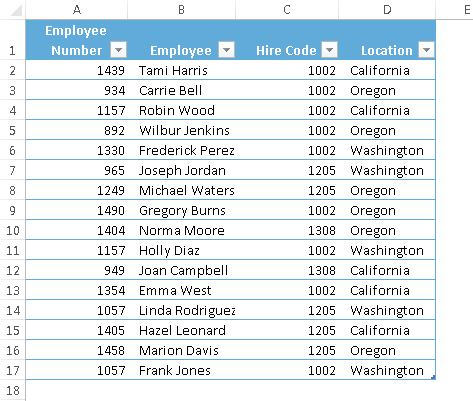
Figure 14-3:
Indenting the text makes the table easier to read.
Tip 15: Using Named Styles
Throughout the years, one of the most underused features in Excel has been named styles. Named styles make it very easy to apply a set of predefined formatting options to a cell or range. In addition to saving time, using named styles helps to ensure a consistent look across your worksheets.
A style can consist of settings for up to six different attributes (which correspond to the tabs in the Format Cells dialog box):
→ Number format
→ Alignment (vertical and horizontal)
→ Font (type, size, and color)
→ Borders
→ Fill (background color)
→ Protection (locked and hidden)
The real power of styles is apparent when you change a component of a style. All cells that have been assigned that named style automatically incorporate the change. Suppose that you apply a particular style to a dozen cells scattered throughout your worksheet. Later, you realize that these cells should have a font size of 14 points rather than 12 points. Rather than change each cell, simply edit the style definition. All cells with that particular style change automatically.
Using the Style gallery
Excel comes with dozens of predefined styles, and you apply these styles in the Style gallery (located in the Home⇒Styles group). Figure 15-1 shows the predefined styles in the Style gallery. To apply a style to the selected cell or range, just click the style. Notice that this gallery provides a preview. When you hover your mouse over a style, it’s temporarily applied to the selection so that you can see the effect. To make it permanent, just click the style.
After you apply a style to a cell, you can apply additional formatting to it by using any formatting method discussed in this chapter. Formatting modifications that you make to the cell don’t affect other cells that use the same style.
To maximize the value of styles, it’s best to avoid additional formatting. Rather, consider creating a new style (explained later in this tip).
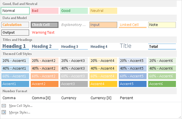
Figure 15-1:
Use the Style gallery to work with named styles.
Modifying an existing style
To change an existing style, activate the Style gallery, right-click the style you want to modify, and choose Modify from the shortcut menu. Excel displays the Style dialog box, shown in Figure 15-2. In this example, the Style dialog box shows the settings for the Normal style, which is the default style for all cells. (The style definitions vary, depending on which document theme is active.)
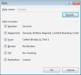
Figure 15-2:
Use the Style dialog box to modify named styles.
Cells, by default, use the Normal style. Here’s a quick example of how you can use styles to change the default font used throughout your workbook:
1.
Choose Home⇒Styles⇒Cell Styles.
Excel displays the list of styles for the active workbook.
2.
Right-click Normal in the Styles list and choose Modify.
The Style dialog box opens with the current settings for the Normal style.
3.
Click the Format button.
The Format Cells dialog box opens.
4.
Click the Font tab and choose the font and size that you want as the default.
5.
Click OK to return to the Style dialog box.
6.
Click OK again to close the Style dialog box.
The font for all cells that use the Normal style changes to the font that you specified. You can change any formatting attributes for any style.
Creating new styles
In addition to using the built-in Excel styles, you can create your own styles. This flexibility can be quite handy because it enables you to apply your favorite formatting options very quickly and consistently.
To create a new style from an existing formatted cell, follow these steps:
1.
Select a cell and apply all the formatting that you want to include in the new style.
You can use any of the formatting that’s available in the Format Cells dialog box.
2.
After you format the cell to your liking, activate the Style gallery and choose New Cell Style.
The Style dialog box opens, along with a proposed generic name for the style. Note that Excel displays the words “By Example” to indicate that it’s basing the style on the current cell.
3.
Enter a new style name in the Style Name box.
The check boxes show the current formats for the cell. By default, all check boxes are checked.
4.
If you don’t want the style to include one or more format categories, remove the check marks from the appropriate boxes.
5.
Click OK to create the style and close the dialog box.
After you perform these steps, the new custom style is available in the Style gallery. Custom styles are available only in the workbook in which they were created. To copy your custom styles, see the section that follows.
 The Protection option in the Styles dialog box controls whether users can modify cells for the selected style. This option is effective only if you also turn on worksheet protection, by choosing Review⇒Changes⇒Protect Sheet.
Merging styles from other workbooks
It’s important to understand that custom styles are stored with the workbook in which they were created. If you created some custom styles, you probably don’t want to go through all the work to create copies of those styles in each new Excel workbook. A better approach is to merge the styles from a workbook in which you previously created them.
To merge styles from another workbook, open both the workbook that contains the styles you want to merge and the workbook into which you want to merge styles. From the workbook into which you want to merge styles, activate the Style gallery and choose Merge Styles. The Merge Styles dialog box opens with a list of all open workbooks. Select the workbook that contains the styles you want to merge and click OK. Excel copies styles from the workbook you selected into the active workbook.
You may want to create a master workbook that contains all your custom styles so that you always know from which workbook to merge styles.
Tip 16: Creating Custom Number Formats
Although Excel provides a good variety of built-in number formats, you may find that none of them suits your needs. In such a case, you can probably create a custom number format. You do so on the Number tab of the Format Cells dialog box (see Figure 16-1). The easiest way to display this dialog box is to press Ctrl+1. Or click the dialog box launcher in the Home⇒Number group. (The dialog box launcher is the small icon to the right of the word
Number.
)
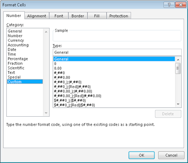
Figure 16-1:
Create custom number formats on the Number tab of the Format Cells dialog box.
Many Excel users — even advanced users — avoid creating custom number formats because they think that the process is too complicated. In reality, custom number formats tend to
look
more complex than they are.
You construct a number format by specifying a series of codes as a number format string. To enter a custom number format, follow these steps:
1.
Press Ctrl+1 to display the Format Cells dialog box.
2.
Click the Number tab and select the Custom category.
3.
Enter your custom number format in the Type field.
See Tables 16-1 and 16-2 for examples of codes you can use to create your own, custom number formats.
4.
Click OK to close the Format Cells dialog box.
Parts of a number format string
A custom format string enables you to specify different format codes for four categories of values: positive numbers, negative numbers, zero values, and text. You do so by separating the codes for each category with a semicolon. The codes are arranged in four sections, separated by semicolons:
Positive format; Negative format; Zero format; Text format
The following general guidelines determine how many of these four sections you need to specify:
→ If your custom format string uses only one section, the format string applies to all values.
→ If you use two sections, the first section applies to positive values and zeros, and the second section applies to negative values.
→ If you use three sections, the first section applies to positive values, the second section applies to negative values, and the third section applies to zeros.
→ If you use all four sections, the last section applies to text stored in the cell.
The following example of a custom number format specifies a different format for each of these types: