Programming Python (98 page)

One
of the first things I always look for when exploring a new
computer interface is a clock. Because I spend so much time glued to
computers, it’s essentially impossible for me to keep track of the time
unless it is right there on the screen in front of me (and even then, it’s
iffy). The next program, PyClock, implements such a clock widget in
Python. It’s not substantially different from the clock programs that you
may be used to seeing on the X Window System. Because it is coded in
Python, though, this one is both easily customized and fully portable
among Windows, the X Window System, and Macs, like all the code in this
chapter. In addition to advanced GUI techniques, this example demonstrates
Pythonmathandtimemodule tools.
Before I show
you PyClock, though, let me provide a little background
and a confession. Quick—how do you plot points on a circle? This, along
with time formats and events, turns out to be a core concept in clock
widget programs. To draw an analog clock face on a canvas widget, you
essentially need to be able to sketch a circle—the clock face itself is
composed of points on a circle, and the second, minute, and hour hands
of the clock are really just lines from a circle’s center out to a point
on the circle. Digital clocks are simpler to draw, but not much to look
at.
Now the confession: when I started writing PyClock, I couldn’t
answer the last paragraph’s opening question. I had utterly forgotten
the math needed to sketch out points on a circle (as had most of the
professional software developers I queried about this magic formula). It
happens. After going unused for a few decades, such knowledge tends to
be garbage collected. I finally was able to dust off a few neurons long
enough to code the plotting math needed, but it wasn’t my finest
intellectual hour.
[
40
]
If you are in the same boat, I don’t have space to teach geometry
in depth here, but I can show you one way to code the point-plotting
formulas in Python in simple terms. Before tackling the more complex
task of implementing a clock, I wrote theplotterGuiscript shown in
Example 11-11
to focus on just the
circle-plotting logic.
Itspointfunction is where the
circle logic lives—it plots the (X,Y) coordinates of a point on the
circle, given the relative point number, the total number of points to
be placed on the circle, and the circle’s radius (the distance from the
circle’s center to the points drawn upon it). It first calculates the
point’s angle from the top by dividing 360 by the number of points to be
plotted, and then multiplying by the point number; in case you’ve
forgotten too, it’s 360 degrees around the whole circle (e.g., if you
plot 4 points on a circle, each is 90 degrees from the last, or 360/4).
Python’s standardmathmodule gives
all the required constants and functions from that point forward—pi,
sine, and cosine. The math is really not too obscure if you study this
long enough (in conjunction with your old geometry text if necessary).
There are alternative ways to code the number crunching, but I’ll skip
the details here (see the examples package for hints).
Even if you don’t care about the math, though, check out
Example 11-11
’scirclefunction. Given the (X,Y) coordinates
of a point on the circle returned bypoint, it draws a line from the circle’s
center out to the point and a small rectangle around the point
itself—not unlike the hands and points of an analog clock. Canvas tags
are used to associate drawn objects for deletion before each
plot.
Example 11-11. PP4E\Gui\Clock\plotterGui.py
# plot circles on a canvas
import math, sys
from tkinter import *
def point(tick, range, radius):
angle = tick * (360.0 / range)
radiansPerDegree = math.pi / 180
pointX = int( round( radius * math.sin(angle * radiansPerDegree) ))
pointY = int( round( radius * math.cos(angle * radiansPerDegree) ))
return (pointX, pointY)
def circle(points, radius, centerX, centerY, slow=0):
canvas.delete('lines')
canvas.delete('points')
for i in range(points):
x, y = point(i+1, points, radius-4)
scaledX, scaledY = (x + centerX), (centerY - y)
canvas.create_line(centerX, centerY, scaledX, scaledY, tag='lines')
canvas.create_rectangle(scaledX-2, scaledY-2,
scaledX+2, scaledY+2,
fill='red', tag='points')
if slow: canvas.update()
def plotter():   # 3.x // trunc div
circle(scaleVar.get(), (Width // 2), originX, originY, checkVar.get())
def makewidgets():
global canvas, scaleVar, checkVar
canvas = Canvas(width=Width, height=Width)
canvas.pack(side=TOP)
scaleVar = IntVar()
checkVar = IntVar()
scale = Scale(label='Points on circle', variable=scaleVar, from_=1, to=360)
scale.pack(side=LEFT)
Checkbutton(text='Slow mode', variable=checkVar).pack(side=LEFT)
Button(text='Plot', command=plotter).pack(side=LEFT, padx=50)
if __name__ == '__main__':
Width = 500                                       # default width, height
if len(sys.argv) == 2: Width = int(sys.argv[1])   # width cmdline arg?
originX = originY = Width // 2                    # same as circle radius
makewidgets()                                     # on default Tk root
mainloop()                                        # need 3.x // trunc div
The circle defaults to 500 pixels wide unless you pass a width on
the command line. Given a number of points on a circle, this script
marks out the circle in clockwise order every time you press Plot, by
drawing lines out from the center to small rectangles at points on the
circle’s shape. Move the slider to plot a different number of points and
click the checkbox to make the drawing happen slow enough to notice the
clockwise order in which lines and points are drawn (this forces the
script toupdatethe display after
each line is drawn).
Figure 11-19
shows the
result for plotting 120 points with the circle width set to 400 on the
command line; if you ask for 60 and 12 points on the circle, the
relationship to clock faces and hands starts becoming clearer.
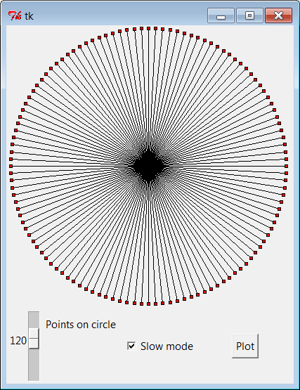
Figure 11-19. plotterGui in action
For more help, this book’s examples distribution also includes
text-based versions of this plotting script that print circle point
coordinates to thestdoutstream for
review, instead of rendering them in a GUI. See the
plotterText.py
scripts in the clock’s
directory
. Here is the sort of output they
produce when plotting 4 and 12 points on a circle that is 400 points
wide and high; the output format is simply:
pointnumber : angle = (Xcoordinate, Ycoordinate)
and assumes that the circle is centered at coordinate
(0,0):
----------
1 : 90.0 = (200, 0)
2 : 180.0 = (0, −200)
3 : 270.0 = (−200, 0)
4 : 360.0 = (0, 200)
----------
1 : 30.0 = (100, 173)
2 : 60.0 = (173, 100)
3 : 90.0 = (200, 0)
4 : 120.0 = (173, −100)
5 : 150.0 = (100, −173)
6 : 180.0 = (0, −200)
7 : 210.0 = (−100, −173)
8 : 240.0 = (−173, −100)
9 : 270.0 = (−200, 0)
10 : 300.0 = (−173, 100)
11 : 330.0 = (−100, 173)
12 : 360.0 = (0, 200)
----------
Numeric Python Tools
If you do enough
number crunching to have followed this section’s
abbreviated geometry lesson, you will probably also be interested in
exploring the
NumPy
numeric programming
extension for Python. It adds things such as vector objects and
advanced mathematical operations, effectively turning Python into a
scientific/numeric programming tool that supports efficient numerical
array computations, and it has been compared to MatLab. NumPy has been
used effectively by many organizations, including Lawrence Livermore
and Los Alamos National Labs—in many cases, allowing Python with NumPy
to replace legacy FORTRAN code.
NumPy must be fetched and installed separately; see Python’s
website for links. On the web, you’ll also find related numeric tools
(e.g., SciPy), as well as visualization and 3-D animation tools (e.g.,
PyOpenGL, Blender, Maya, vtk, and VPython). At this writing, NumPy
(like the many numeric packages that depend upon it) is officially
available for Python 2.X only, but a version that supports both
versions 2.X and 3.X is in early development release form. Besides themathmodule, Python itself also has
a built-in complex number type for engineering work, a fixed-precision
decimal type added in release 2.4, and a rational fraction type added
in 2.6 and 3.0. See the library manual and Python language
fundamentals books such as
Learning
Python
for details.
To understand how these points are mapped to a canvas, you first
need to know that the width and height of a circle are always the
same—the radius × 2. Because tkinter canvas (X,Y) coordinates start at
(0,0) in the upper-left corner, the plotter GUI must offset the circle’s
center point to coordinates (width/2, width/2)—the origin point from
which lines are drawn. For instance, in a 400 × 400 circle, the canvas
center is (200,200). A line to the 90-degree angle point on the right
side of the circle runs from (200,200) to (400,200)—the result of adding
the (200,0) point coordinates plotted for the radius and angle. A line
to the bottom at 180 degrees runs from (200,200) to (200,400) after
factoring in the (0,-200) point plotted.
This point-plotting algorithm used byplotterGui, along with a few scaling
constants, is at the heart of the PyClock analog display. If this still
seems a bit much, I suggest you focus on the PyClock script’s
digital
display implementation first; the analog
geometry plots are really just extensions of underlying timing
mechanisms used for both display modes. In fact, the clock itself is
structured as a genericFrameobject
that
embeds
digital and analog display objects and
dispatches time change and resize events to both in the same way. The
analog display is an attachedCanvasthat knows how to draw circles, but the digital object is simply an
attachedFramewith labels to show
time
components.
Apart from the
circle geometry bit, the rest of PyClock is
straightforward. It simply draws a clock face to represent the current
time and uses widgetaftermethods to
wake itself up 10 times per second to check whether the system time has
rolled over to the next second. On second rollovers, the analog second,
minute, and hour hands are redrawn to reflect the new time (or the text
of the digital display’s labels is changed). In terms of GUI
construction, the analog display is etched out on a canvas, redrawn
whenever the window is resized, and changes to a digital format upon
request.
PyClock also puts Python’s standardtimemodule into service to fetch and convert
system time information as needed for a clock. In brief, theonTimermethod gets system time withtime.time, a built-in tool that returns a
floating-point number giving seconds since the
epoch
—the point from which your computer counts
time. Thetime.localtimecall is then
used to convert epoch time into a tuple that contains hour, minute, and
second values; see the script and Python library manual for additional
details.
Checking the system time 10 times per second may seem intense, but
it guarantees that the second hand ticks when it should, without jerks
or skips (afterevents aren’t
precisely timed). It is not a significant CPU drain on systems I use. On
Linux and Windows, PyClock uses negligible processor resources—what it
does use is spent largely on screen updates in analog display mode, not
onafterevents.
[
41
]
To minimize screen updates, PyClock redraws only clock hands on
second rollovers; points on the clock’s circle are redrawn only at
startup and on window resizes.
Figure 11-20
shows the default initial
PyClock display format you get when the file
clock.py
is run directly.
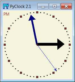
Figure 11-20. PyClock default analog display
The clock hand lines are given arrows at their endpoints with the
canvas line object’sarrowandarrowshapeoptions. Thearrowoption can befirst,last,none,
orboth; thearrowshapeoption takes a tuple giving the
length of the arrow touching the line, its overall length, and its
width.
Like PyView, PyClock also uses the widgetpack_forgetandpackmethods to dynamically erase and redraw
portions of the display on demand (i.e., in response to bound events).
Clicking on the clock with a left mouse button changes its display to
digital by erasing the analog widgets and drawing the digital interface;
you get the simpler display captured in
Figure 11-21
.
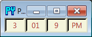
Figure 11-21. PyClock goes digital
This digital display form is useful if you want to conserve real
estate on your computer screen and minimize PyClock CPU utilization (it
incurs very little screen update overhead). Left-clicking on the clock
again changes back to the analog display. The analog and digital
displays are both constructed when the script starts, but only one is
ever packed at any given time.
A right mouse click on the clock in either display mode shows or
hides an attached label that gives the current date in simple text form.
Figure 11-22
shows a
PyClock running with an analog display, a clicked-on date label, and a
centered photo image object (this is clock style started by the
PyGadgets launcher):
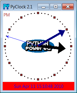
Figure 11-22. PyClock extended display with an image
The image in the middle of
Figure 11-22
is added by passing
in a configuration object with appropriate settings to the PyClock
object constructor. In fact, almost everything about this display can be
customized with attributes in PyClock configuration
objects—
hand colors, clock tick colors,
center photos, and initial size.
Because PyClock’s analog display is based upon a manually sketched
figure on a canvas, it has to process window
resize
events itself: whenever the window shrinks or expands, the clock face
has to be redrawn and scaled for the new window size. To catch screen
resizes, the script registers for thebind; surprisingly, this isn’t a top-level
window manager event like the Close button. As you expand a PyClock, the
clock face gets bigger with the window—try expanding, shrinking, and
maximizing the clock window on your computer. Because the clock face is
plotted in a square coordinate system, PyClock always expands in equal
horizontal and vertical proportions, though; if you simply make the
window only wider or taller, the clock is unchanged.
Added in the third edition of this book is a countdown timer
feature: press the “s” or “m” key to pop up a simple dialog for entering
the number of seconds or minutes for the countdown, respectively. Once
the countdown expires, the pop up in
Figure 11-23
appears and fills
the entire screen on Windows. I sometimes use this in classes I teach to
remind myself and my students when it’s time to move on (the effect is
more striking when this pop up is projected onto an entire
wall!).
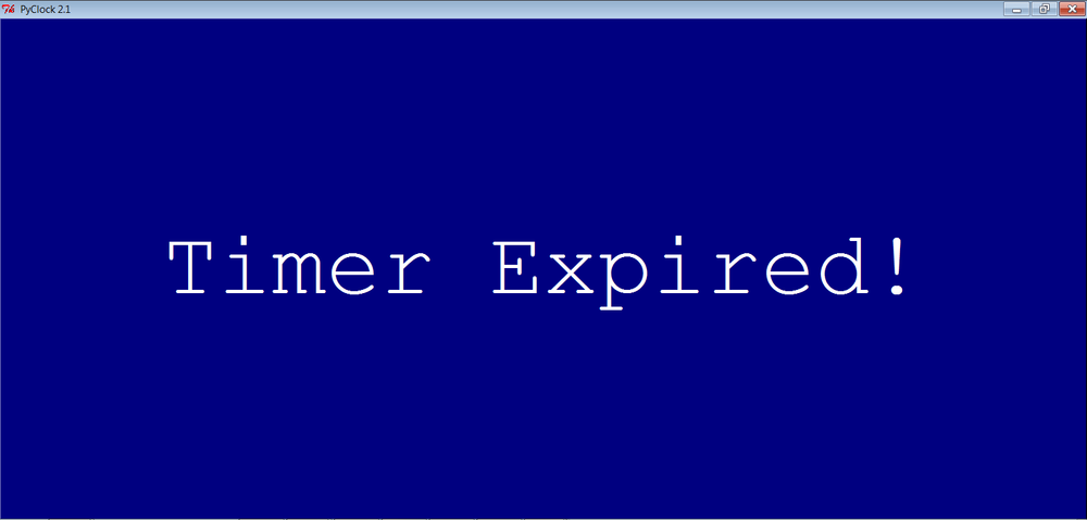
Figure 11-23. PyClock countdown timer expired
Finally, like PyEdit, PyClock can be run either standalone or
attached to and embedded in other GUIs that need to display the current
time. When standalone, thewindowsmodule from the preceding chapter (
Example 10-16
) is reused here to
get a window icon, title, and quit pop up for free. To make it easy to
start preconfigured clocks, a utility module calledclockStylesprovides a set of clock
configuration objects you can import, subclass to extend, and pass to
the clock constructor;
Figure 11-24
shows a few of the
preconfigured clock styles and sizes in action, ticking away in
sync.
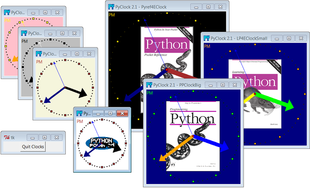
Figure 11-24. A few canned clock styles: clockstyles.py
Run
clockstyles.py
(or select
PyClock from PyDemos, which does the same) to recreate this timely scene
on your computer. Each of these clocks usesafterevents to check for system-time rollover
10 times per second. When run as top-level windows in the same process,
all receive a timer event from the same event loop. When started as
independent programs, each has an event loop of its own. Either way,
their second hands sweep in unison each
second.